

Abstract
Normal eye movements ensure that the visual world is seen episodically, as a series of often stationary images. In this paper we characterize the responses of neurons in striate cortex to stationary grating patterns presented with abrupt onset. These responses are distinctive. In most neurons the onset of a grating gives rise to a transient discharge that decays with a time constant of 100 msec or less. The early stages of response have higher contrast gain and higher response gain than later stages. Moreover, the variability of discharge during the onset transient is disproportionately low. These factors together make the onset transient an information-rich component of response, such that the detectability and discriminability of stationary gratings grows rapidly to an early peak, within 150 msec of the onset of the response in most neurons. The orientation selectivity of neurons estimated from the first 150 msec of discharge to a stationary grating is indistinguishable from the orientation selectivity estimated from longer segments of discharge to moving gratings. Moving gratings are ultimately more detectable than stationary ones, because responses to the former are continuously renewed. The principal characteristics of the response of a neuron to a stationary grating—the initial high discharge rate, which decays rapidly, and the change of contrast gain with time—are well captured by a model in which each excitatory synaptic event leads to an immediate reduction in synaptic gain, from which recovery is slow.
- visual cortex
- striate cortex
- detectability (d')
- discriminability
- variability
- reliability
- refractoriness
- mean-to-variance ratio
- contrast gain
- gain control
- orientation selectivity
- synaptic depression
Natural viewing of scenes brings about a series of episodic image exposures, many of them to stationary objects. Most cells in striate cortex (V1) respond sharply but transiently to the onset of a stationary pattern (Tolhurst et al., 1980), with a discharge the time course of which is unlike that elicited by the moving gratings often used in quantitative studies of cortical neurons. Moving gratings evoke a continuous discharge that is modulated (simple cells) or nearly uniform (complex cells).
The brevity of fixations in many tasks [often <200 msec (Epelboim et al., 1994)] implies that observers obtain information quickly; measurements of integration time for resolution and vernier acuity (Keesey, 1960) show that performance becomes asymptotically good for exposure durations of <200 msec; for stereoacuity (Shortess and Krauskopf, 1961), asymptote is reached between 250 and 500 msec. These observations encourage the notion that the early part of the response of a neuron to an unchanging stimulus will be especially important (Zohary et al., 1990; Tovée et al., 1993).
In this paper we explore the early stages of the responses of V1 neurons to visual stimuli. We characterize the development of responsivity and of stimulus selectivity and the reliability with which neurons can distinguish different stimuli. We find that in most neurons the earliest stages of response have distinctively high gain, and often low noise, permitting neurons to achieve rapidly their highest sensitivity and sharpest selectivity—so much so that the reliability with which a cell signals a stimulus is sometimes diminished by attending to parts of response beyond the initial transient. We develop a model to account for the transient responses.
MATERIALS AND METHODS
Preparation and recording. Experiments were undertaken on 11 Macaca fascicularis that weighed between 2.5 and 5 kg. Each animal was anesthetized initially with ketamine hydrochloride (Vetalar; 10 mg/kg, i.m.). Cannulas were inserted into the saphenous veins, and the trachea was cannulated. Surgery was continued under sufentanil citrate (Sufenta) anesthesia. In anesthetic doses, Sufenta often produces severe respiratory depression, so animals were artificially ventilated after its administration. The head was placed in a stereotaxic frame, and a craniotomy 10 mm in diameter was made near the representation of the fovea, centered ∼5 mm behind the lunate sulcus. Electrodes were attached to the exposed skull to monitor the electroencephalogram (EEG) and to the forearms to monitor the electrocardiogram (ECG). No procedure (other than the initial injection) was undertaken without anesthesia; all procedures conformed to the most recent recommendations published by the National Institutes of Health (NIH, 1991).
After surgery, anesthesia was maintained by a continuous infusion of Sufenta (initially 4 mg · kg−1 · hr−1) in a mixture of lactated Ringer's solution and dextrose. The adequacy of this dose was ensured by observing the monkey for 3 hr before administering muscle relaxant. The dose was increased if the animal showed any signs of arousal. To prevent eye movements, a loading dose of vecuronium bromide (Norcuron) was infused rapidly and was followed by a continuous infusion at 100 mg · kg−1 · hr−1. The monkey was ventilated at 20 strokes per minute at a tidal volume adjusted to keep the end-tidal CO2 close to 33 mmHg. The EEG and ECG were monitored continuously, and at any sign of arousal the anesthetic dose was increased. A heating blanket controlled by a subscapular thermistor kept body temperature near 37°C.
Pupils were dilated with atropine sulfate, and the corneas were protected with high-permeability clear contact lenses (Fluroperm 92). These remained in place for the duration of the experiment. Artificial pupils 3 mm in diameter were placed in front of the eyes. Supplementary lenses were usually required to focus stimuli on the retina; these were chosen as a result of an ophthalmoscopic exam. At the beginning of the experiment, and each time the eyes were examined, the foveal reflex was found and projected by reversed ophthalmoscopy onto a tangent screen 1.3 m in front of the animal.
Just before recording began, a small slit was made in the exposed dura, into which was passed a guide tube containing the electrode. After the electrode carrier had been positioned, the dura was covered with warm agar and sealed with dental acrylic. Action potentials were recorded with glass-insulated tungsten microelectrodes (Merrill and Ainsworth, 1972) positioned with a stepping motor-driven micrometer. Near-vertical penetrations were made through striate cortex containing the representation of the central 3°. An electrolytic lesion was made at the end of each penetration, and further lesions were made at irregular intervals during withdrawal of the electrode. This helped identify penetrations unambiguously. At the end of the experiment the monkey was perfused through the heart with 0.9% saline in neutral phosphate buffer, followed by a solution of 10% paraformaldehyde. The brain was blocked and sunk in 30% sucrose, after which it was frozen and cut into 50 μm sections that were stained for Nissl substance. Electrode tracks were reconstructed from the fixed tissue.
Visual stimuli. Sinusoidal gratings were generated by a Macintosh computer on a television monitor displaying 832 × 640 pixels at 28.3 pixels per centimeter. The screen was refreshed at 75 Hz. At the viewing distances used (which varied between 114 and 342 cm according to the resolving power of the neuron under study), the width of the screen subtended between 14.5° (57 pixels per degree) and 4.9° (170 pixels per degree). To generate a grating, a static saw-tooth waveform of the appropriate spatial frequency, orientation, and size was drawn in video memory. The type of waveform displayed (sinusoid, square wave, etc.), its movement or flicker, and its color and contrast were controlled by manipulation of video lookup table entries. Multiple, independently controlled gratings could be displayed simultaneously. Lookup tables could be rewritten completely during frame fly-back. The space–time average luminance was constant, and when no grating was visible the screen displayed a spatially uniform field of the average luminance. For early experiments we used a Nanao T560i monitor (mean luminance 48 cd/m2) driven by a RasterOps ProColor 32 video board with lookup tables that provided 256 values per channel with nine-bit resolution. In later experiments we used an NEC P750 monitor (mean luminance 54 cd/m2) driven by a Radius ThunderPower 1920 video board with lookup tables that provided 256 values per channel with 10-bit resolution. Calibration and correction of the nonlinear relationship between voltage and luminance cost ∼0.5 bits of resolution.
In most experiments a neuron was stimulated with a series of gratings that differed along one or more dimensions (e.g., orientation, spatial frequency). In such cases, the different stimuli in a set were presented in pseudorandom order, and all members of the set were displayed once before the cycle was repeated (with a different order). A single experiment could contain up to 40 presentation cycles. When moving gratings were used, the temporal frequency was between 2 and 8 Hz, chosen to be near the optimum for the cell under study. All gratings, whether moving or stationary, were presented monocularly, with abrupt onset and offset.
Measurement of response. The analog signal recorded by the electrode was amplified, filtered, and digitized, then scrutinized in real time for voltage excursions that might represent action potentials. Putative spikes were displayed on the computer monitor, and templates for discriminating spikes were constructed by averaging multiple traces. After templates had been formed, the times of the leading edges of action potentials were recorded with a precision of 100 μsec, tagged with a spike identifier, and placed in a queue that was synchronized with the stimulus event queue.
In early experiments the analog sampling (at 10 kHz) was controlled by a digital signal processor (National Instruments NB-DSP2300) in a Macintosh Quadra 950 computer. The digital signal processor also analyzed the waveform to extract the candidate spikes and undertook the template matching to capture spikes. In later experiments, using a dual processor Power Macintosh 9600, the analog signal was recorded directly by the sound input manager (at 44.1 kHz, subsampled to 11.025 kHz), and the second processor analyzed the recorded waveform and generated the queue of spike times. This was available for real-time analysis during the experiment and was saved for off-line analysis.
Characterizing receptive fields. Receptive fields were first mapped using a small patch of moving grating the spatial and temporal characteristics of which were continuously adjustable by the experimenter. Having obtained a preliminary estimate of the preferred position, size, orientation, and spatial frequency of the neuron, we then used a standard protocol, involving randomly interleaved presentations of different moving gratings, to establish first the orientation tuning, then the spatial frequency tuning, and then (using gratings of optimal orientation and spatial frequency) the contrast–response relationship. From the latter measurement we chose a contrast at which we could present stimuli without eliciting responses of saturating amplitude. This permitted us to see clearly any variations in responsivity that resulted from subsequent stimulus variations. The position of the receptive field was established using a patch of moving grating, of length and width approximately matching the receptive field, presented at a matrix of positions centered on the estimated position and spaced 0.25 lengths and widths apart. Having found the receptive field position, we then established the rectangle (lying in the preferred orientation of the neuron) that best matched the receptive field in size. To establish the optimal length we used a series of gratings of different lengths and widths fixed at a preliminary estimate; to establish the preferred width we used a series of gratings of different widths, with length fixed at the length preferred. If at any stage in this sequence of measurements it appeared that some estimate was incorrect, we repeated the sequence.
For the basic measurements, each grating in the stimulus set was presented for 1.25 sec, in a random sequence with all the others. The screen was blank for 0.75 sec between presentations. The whole cycle was repeated (in different random order) as many times as were needed to characterize reliably the properties of the neuron. This could be as many as 20 times but was usually fewer.
For experiments that required the use of stationary gratings, we made additional preliminary measurements, using unmodulated gratings, to establish the optimal spatial phase of the grating. This was particularly important for work on simple cells and less so for complex cells. Spatial phase was defined relative to the center of the grating patch.
Statistical analysis. To establish whether responses from a population of n neurons to stimuli of two classes differed reliably, we used permutation tests (Edgington, 1995). In each case the null hypothesis was that responses of all neurons to both stimuli came from a single distribution. A simulated data set was drawn randomly from that distribution by choosing each of the 2n actual responses without replacement. This was repeated 5000 times. To assess statistical significance we computed a p value, the probability that a mean signed difference between responses to the two stimulus classes in a simulated data set was greater than or equal to that for the actual data. A similar permutation test was used to compute the statistical significance of correlation coefficients.
RESULTS
We recorded action potentials from 43 simple cells and 83 complex cells in V1 of 11 monkeys. Simple and complex cells behaved similarly in most of the measurements we describe, so are distinguished only where their behaviors differ. Among the neurons for which locations were identified (most lay in layer II/III), no distinctive variations in the character of the responses to stationery stimuli were associated with the layer of origin.
Time course of response
Figure 1 shows the responses of two V1 cells to stationary gratings of optimal orientation, spatial frequency, phase, and size, presented for 1250 msec. The trace below defines the time course of the stimuli. The initially brisk responses decline quickly. These declines, which are characteristic of cortical neurons, are consistent with the low sensitivity to low temporal frequencies found by Hawken et al. (1996), although nonlinearities in the behavior of cortical neurons make the decay of responses to steps even more rapid and complete than would be expected from the temporal modulation transfer function (MTF) (Tolhurst et al., 1980; Chance et al., 1998). The discharge is less sustained than would be predicted by the shallow low-frequency tails of the temporal MTF of parvocellular retinal ganglion cells (Purpura et al., 1990) or lateral geniculate nucleus (LGN) neurons (Hawken et al., 1996). V1 neurons also adapt rapidly after stimulus onset (Müller et al., 1999), a behavior not seen in LGN, and rapid cortical adaptation has been found to have a time course that closely matches that of initial declines in response, suggesting that cortical adaptation may be responsible for declines in response (Lisberger and Movshon, 1999). All this suggests that although LGN neurons will contribute to the declines in Figure 1, they must also depend substantially on some mechanism within cortex.

Average responses of two V1 cells (irregular traces) to the presentation of a stationary grating of optimal orientation, spatial frequency, phase, and size. Histograms have a bin width of 10 msec. The trace below defines the time course of the stimulus. Smooth curves drawn through the data are best fits of the synaptic depression model described in Discussion. A, Simple cell, 20 repetitions. Model parameter values are Vstim, 0.25 mV;d, 0.99; τ, 600 msec; τpsp, 20 msec; L, 70 msec; (Vrest− Vthresh), −0.1 mV;S, 1.1 (imp/sec)/mV. B, Complex cell, nine repetitions. Model parameter values areVstim, 0.25 mV; d, 0.98; τ, 175 msec; τpsp, 10 msec;L, 40 msec; (Vrest −Vthresh), −0.1 mV; S, 4.3 (imp/sec)/mV.
The discharge rate R after the initial peak is well described by an exponential decay (fit not shown):
 Equation 1where Rmax is the peak discharge rate, Rmin is the asymptotic discharge rate during stimulus presentation, τ is the time-constant of decay, and t is the time since peak. The decaying discharge can be conveniently characterized by its time-constant τ and by the ratioRmin/Rmax, which represents the extent to which the response is sustained. To allow for cases in which Rmin lies below the maintained discharge, we compute the ratio (Rmin −M)/(Rmax −M), where M is the maintained discharge in the absence of a grating. Figure 2summarizes these measures for the neurons we have characterized. Most responses decline quickly to low sustained rates.

Characteristics of the transient responses of a neuron to stationary gratings. A, Distribution of time-constants of the decay of response.B, Distribution of the ratio (Rmin −M)/(Rmax −M).
Characteristics of onset transients
The transient component of the response that follows the onset of a stationary grating is often prominent and can provide a substantial fraction of the impulses ever evoked by the grating. To better appreciate the importance of this, we explored the development of stimulus selectivity and the size and variability of the discharge of a neuron as a function of contrast, at different times during the response to a stationary grating.
Stimulus selectivity
Figure 3 shows, for two neurons (inA the neuron from Fig. 1A), the orientation tuning for stationary gratings, estimated from the complete response to a 1250 msec presentation (○, dashed traces) and the first 50 msec of response (●, solid traces). Both measures yield the same preferred orientation and selectivity. The tuning curve based on responses accumulated for 50 msec is as reliable as that based on responses accumulated for 1250 msec (evident in the error bars, which show ±1 SEM). The spatial frequency tuning of a neuron develops equally rapidly (data not shown).

Orientation tuning of a simple cell (A) and a complex cell (B), estimated from the first 50 msec of discharge (●, solid traces) and the complete response (○, dashed traces) to the presentation of a stationary grating for 1250 msec. Graphs are normalized to the average discharge rate for the preferred orientation. Actual discharge rates for the preferred orientations were as follows: for the first 50 msec, 82 imp/sec (A) and 60 imp/sec (B); for the complete 1250 msec of response, 39 imp/sec (A) and 5 imp/sec (B).Ascending vertical bars show +1 SEM of the mean response for the first 50 msec; descending bars show −1 SEM of the mean response for the entire 1250 msec presentation.A shows tuning of the neuron in Figure1A.
Contrast–response relations
The transient discharge after the onset of a stationary grating implies that the responsivity (impulses per unit contrast) of a neuron changes rapidly. This can be seen by comparing contrast–response relations measured during the peak of the response and at a later stage when response has decayed. Figure 4,A and B, illustrates this for one cell. We took two 100 msec segments of discharge, one starting at the beginning of the response and straddling the peak, the other starting 500 msec later (Fig. 4A), and then for each we derived the relation between grating contrast and response amplitude (Fig.4B). Circles show the relation derived from the segment of discharge straddling the peak; squaresshow the relation for the later segment. Figure 4, C andD, shows the corresponding relations for two other neurons.

Contrast–response relations obtained at different times during the response to a stationary grating. A, Responses of one neuron to stationary gratings of contrasts: 100% (top dashed trace) and 50% (bottom dashed trace). Histograms have a bin width of 20 msec. Shaded bars show segments of response from which contrast–response relationships were derived. B–D, Contrast–response relationships for three neurons, derived as inA, at onset (●) and 500 msec later (▪) (neuron inB is the same as A.) Continuous lines drawn through the data are fits of the synaptic depression model described in Discussion. For the neuron inA and B, model parameters are as follows:Vstim, 0.24 mV; d, 0.980; τ, 128 msec; τpsp, 10 msec;L, 50 msec; (Vrest −Vthresh), −0.116 mV;S, 3.80 (imp/ sec)/mV. For the neuron inC, parameters areVstim, 0.6 mV, d, 0.971; τ, 90 msec; τpsp, 10 msec;L, 50 msec; (Vrest −Vthresh), −0.12 mV;S, 4 (imp/sec)/mV (the model fails to account for saturation). For the neuron in D, parameters areVstim, 0.74 mV; d, 0.989; τ, 182 msec; τpsp, 10 msec;L, 50 msec; (Vrest −Vthresh), −0.0342 mV;S, 1.17 (imp/sec)/mV. The model curves inB and to some extent C shift to the right over time; the curve in D does not, because the resting potential of the neuron lies close to threshold. (Vrest −Vthresh)/Vstimis near zero.
The decaying response could reflect a loss of contrast gain (a rightward shift of the contrast–response relation, apparently what happens to the cell of Fig. 4B) or a loss of responsivity (a scaling down, apparently what happens to the cell of Fig. 4D), or both. We can obtain some insight into which change better describes the behavior of our population of cells by using a simple expression to fit the curves and then asking how its parameters change from the peak to the plateau of the response.
The response R to a stimulus of contrast c is often characterized by:
 Equation 2where Rmax
is the response to a high-contrast stimulus after subtracting M, the maintained discharge; n and c50 are parameters that define the steepest slope of the contrast–response function and the contrast about which the steepest portion is centered (Albrecht and Hamilton, 1982). To understand the nature of the changes occurring during the decay of discharge, we have used Equation 2 to characterize pairs of contrast–response relations of the kind shown in Figure 4.
Equation 2where Rmax
is the response to a high-contrast stimulus after subtracting M, the maintained discharge; n and c50 are parameters that define the steepest slope of the contrast–response function and the contrast about which the steepest portion is centered (Albrecht and Hamilton, 1982). To understand the nature of the changes occurring during the decay of discharge, we have used Equation 2 to characterize pairs of contrast–response relations of the kind shown in Figure 4.
For each of 64 neurons, we made least-squares fits of Equation 2 (fits not shown) to the set of responses of each neuron in a single operation, with the exponent n always constrained to have a common value for both curves. In addition, eitherc50 (contrast gain) orRmax (response gain) was constrained to a common value. When c50 was constrained and Rmax was allowed to vary independently, Equation 2 accounted for all but 2.8% of the variance in contrast–response measurements made on the population (that is, the squared difference between the data and model of a neuron was on average 2.8% of the squared difference between the individual data points and the grand mean of all the data points to which the model was fit). For our population of cells, c50was 1.9 ± 2.1, n was 2.5 ± 1.6, andRmax was 138 ± 146 at onset, falling to 65 ± 86 500 msec later. WhenRmax was constrained andc50 was allowed to vary independently, Equation 2 accounted for all but 4.5% of the variance. For our population of cells, Rmax was 153 ± 190, n was 2.3 ± 1.6, andc50 was 1.7 ± 1.8 at onset, and increased to 3.7 ± 2.7 500 msec later. Figure5 shows that for most neurons, variations in c50 andRmax were interchangeable: both constrained fits accounted equally well for the data. This happens because in many neurons the contrast–response relation does not saturate, but continues to grow at high contrasts. Equation 2 then does not provide a well constrained description of the contrast–response relation: variations in c50 andRmax become interchangeable and can be surprisingly large.

For a population of neurons, comparison of error when pairs of contrast–response relations of the kind shown in Figure4 are fit with Equation 2 in a single operation that allows only response gain (Rmax) or only contrast gain (c50) to vary over time. The exponent n is always constrained to have a common value for both curves. Least-squared fit error is given as the percentage of the variance of the data that is not accounted for: that is, the squared difference between the data from a neuron and its model are computed as a percentage of the squared difference between the individual data points and the grand mean of all data points.
For some neurons one fit was superior: sometimes the one that heldRmax to a common value and allowedc50 to vary independently, but more often the one that held c50 to a common value and allowed Rmax to vary independently. It appears that the onset transient has both high contrast gain (lowc50) and high response gain (highRmax), to extents that vary from neuron to neuron. We return to this issue in Discussion, where we develop a model that accounts for both.
Variability of discharge
Previous work has shown that in the steady-state response to a moving grating, the trial-to-trial variance of discharge is generally proportional to the mean spike count (Tolhurst et al., 1983; Shadlen and Newsome, 1998). This appears not to be true of the early stages of responses to stationary gratings. The solid and dotted traces in the post-stimulus time histograms of Figure6A,C,Eshow, for each of three neurons stimulated at 100% contrast, the mean and SD of the spike counts in each bin. The SDs are only slightly higher during the onset transient than at later times when the response has decayed substantially. Figure6B,D,F shows, for each cell, how variance grows with response amplitude, measured over 20 msec segments of discharge at the peak of the response of each neuron (○,solid traces) and 500 msec later (●, dashed traces). Mean spike count is manipulated by presenting the preferred grating of a neuron at a range of contrasts. In both sampling periods the variance grows approximately with the mean when responses are weak, but during the initial transient, variance saturates or declines when responses are strong. This relationship between variance and mean spike count has the same form when computed from 100 msec segments of response.

Relationship between mean rate and variability of discharge in three neurons, one simple (A,B) and two complex (C, Dand E, F). A,C, E, Post-stimulus time histograms showing the mean response to a stationary grating at 100% contrast (solid traces) and its SD (dashed traces), computed for 20 msec bins, calculated over 18–20 trials. SDs are only slightly higher during the onset transient than at later times when the responses have decayed substantially.B, D, F, Response variance plotted against response amplitude, for the neurons inA, C, and E, respectively. Each graph shows the variance in 20 msec segments of discharge, measured at the peak of the response of each neuron (usually ∼30 msec after response onset) (○, solid traces) and 500 msec later (●, dashed traces), against the mean firing rate during the same segments of discharge. Discharge rate is manipulated by presenting the grating preferred by a neuron at a range of contrasts.
Figure 7A compares, for 63 neurons, the ratio of mean (μ) to variance (ς2) in these two 20 msec segments of response to stationary gratings at 100% contrast. The histogram on theright shows the distribution of μ/ς2 for the onset transient (geometric mean 1.8, median 1.6); the histogram above shows the corresponding distribution at 500 msec post-stimulus time (geometric mean 1.1, median 1.1). Distributions of μ/ς2 in 100-msec-long segments of discharge taken early and late in the response differ in the same way as those shown in Figure 7A.
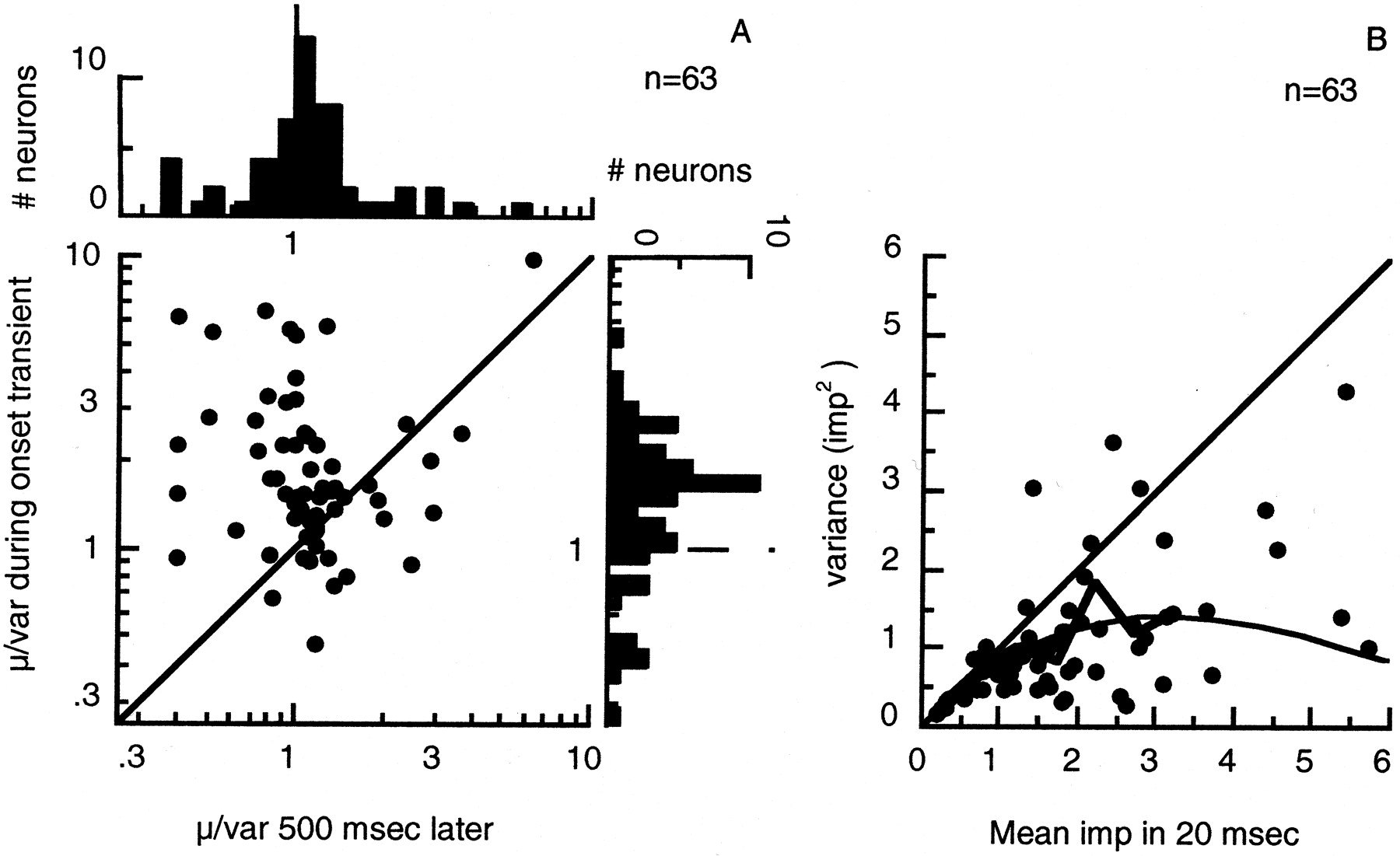
A, Comparison of ratio of mean (μ) to variance (ς2) of discharge during 20 msec segments of response to a stationary grating at 100% contrast, recorded at the peak of the response of a neuron (usually ∼30 msec after response onset) and 500 msec later, for 63 neurons. The histogram on the right shows the distribution of ratios measured during the onset transient (geometric mean 1.8, median 1.6); the histogram above shows the corresponding distribution 500 msec after stimulus onset (geometric mean 1.1, median 1.1). B, Scatter plot showing the variance of discharge during 20 msec samples of discharge recorded at the peak of the response, against the average number of impulses in the samples, for the population. The irregular line traces the average variance in groups of samples aggregated by mean number of impulses in bins 0.5 impulses wide (shown only for bins containing four or more neurons). The diagonal is the relationship expected between variance and mean were spikes generated by a Poisson process. The smooth curve is the relationship expected from a Poisson process limited by an absolute (rectangular) refractory period of 2.25 msec (Barberini et al., 2001).
Several indicators suggest that the relatively low variance during the onset transient results from increased regularity of interspike intervals imposed by an essential refractory period. First, during the onset transient μ/ς2 is disproportionately high only for large responses elicited by high-contrast stimuli (Fig.6B,D,F). Second, when segments of response recorded at onset and later have similar mean amplitude, they have similar μ/ς2. We obtain further insight into this by comparing the variance with the mean at the peak of the response, for the same population of cells (Fig. 7B). The greater the mean number of impulses (or equivalently, the shorter the average interspike interval) in the onset transient, the more variance is reduced below that expected of a Poisson process (diagonal line). This would be expected were firing limited by refractoriness. We return to this in Discussion.
The (often) disproportionately low variability of discharge during the onset transient, coupled with the high responsivity, makes the initial response a potentially rich source of reliable information about the presence of a stimulus. It therefore ought to be an important determinant of the detectability and discriminability of gratings.
Growth of detectability
To examine how important the onset transient might be for stimulus detection, we assume that an ideal observer knows when stimuli are presented (e.g., at the beginning of a fixation) and when to start to integrate the response of a neuron. Because the signal-to-noise ratio is high initially, it will be best to begin integrating at the onset of the response of a neuron, which we identify as the time at which the average discharge rate in response to a stimulus rises above the spontaneous rate (determined by inspection of the post-stimulus time histogram). This was generally between 40 and 80 (mode 50) msec after stimulus onset.
To establish the width of the optimal integration window, we estimated the cumulative detectability of different gratings from samples of response of different durations, beginning at response onset. As a measure of detectability we calculated the capacity of the neuron to distinguish the number of impulses discharged during presentation of a stimulus from the number present in the maintained discharge in the absence of the stimulus. The distribution of impulses in response to a given stimulus was always approximately Gaussian, so we can define the statistic d' as the difference between the means, divided by the SD. When the two distributions had different SDs, we used the root-mean-square SD; thus:
 Equation 3(Green and Swets, 1966). d' is monotonically related to the mutual information that a Gaussian distribution of impulse counts provides about whether a stimulus is present or absent,I = (1/2) log2(1 +d'2) (Rieke et al., 1997). When d' = 0, an ideal observer, given two alternatives, will detect the stimulus correctly on 50% of trials; whend' = 1, it will be 76% correct; when d' = 2, it will be 92% correct.
Figure 8 shows, for the same neurons as Figure 1, how the detectability of an optimal grating grows with the duration of the sample of discharge accumulated from response onset until the time indicated on the abscissa. The different traces in each graph were obtained with gratings of three different contrasts, the lowest being near the contrast that was reliably detected on 75% of trials.
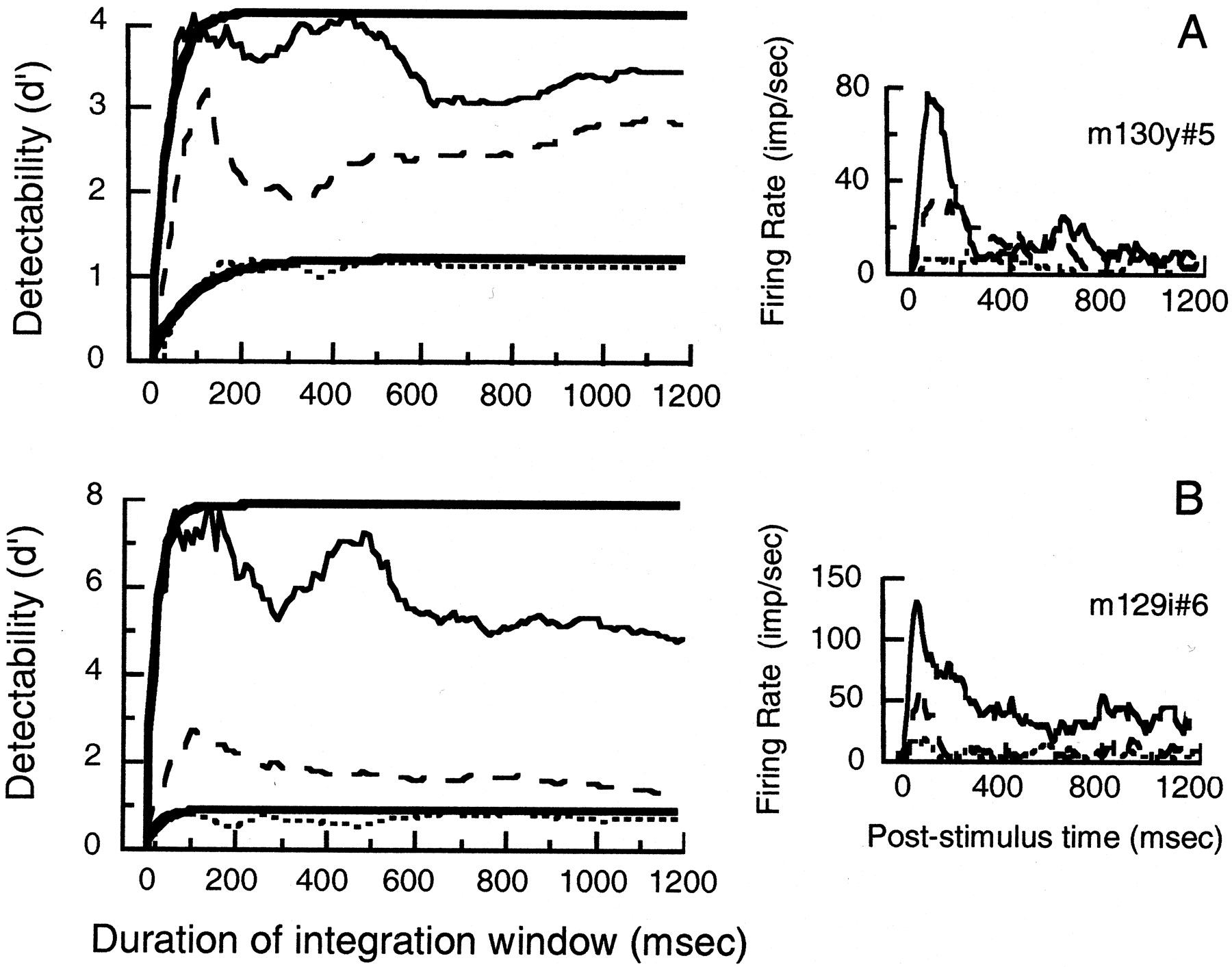
Growth of cumulative detectability (d') of gratings with time from response onset, in two neurons. Each neuron was presented with a stationary grating of optimal spatial frequency and orientation at a range of contrasts including the lowest tested contrast that evoked a reliably detectable response.A, 100% (irregular solid trace), 50% (dashed trace), and 25% (dotted trace).B, 100% (irregular solid trace), 6% (dashed trace), and 3% (dotted trace).Smooth traces, where shown, are exponential fits to the rising portions of the responses (see Eq. 4). Inset histograms to the right of each panel show average discharge from the start of the response, from which time detectability was calculated, smoothed with an exponential decay (asymmetric, causal filter) with a time-constant of 30 msec. Same neurons as Figure 1.
For the cell in Figure 8A, a grating of near-threshold contrast reaches its greatest detectability in 170 msec; at high contrast it reaches its greatest detectability in 80 msec. For the cell in Figure 8B, detectability develops briskly even at low contrast. Figure 8 shows that detectability does not continually improve with increasing length of stimulus presentation: for both neurons the detectability of the grating grows to a peak, then becomes stable or declines. Even for the more sustained responses to gratings of low contrast, detectability stabilizes after an early peak.
The loss of detectability after an initial peak would be surprising if responses were sustained, but responses are transient, falling quickly to near the spontaneous discharge in the absence of a grating (Fig. 8,insets), so integrating spikes beyond the onset transient is much like integrating spikes after the stimulus has been turned off. This can be seen by examining post-stimulus time histograms and SDs of responses. Consider the histogram of Figure 6A, in which during the onset transient the peak count is 2.8 impulses, and the SD is 1.1, so d' is high. Beyond the transient, the mean and SD are both ∼0.75, so by extending the interval of accumulation the signal is diluted more than the noise, and detectability falls. We see this also in Figure 8 and in many other neurons. Figure 9 (solid trace) shows that for the population of neurons as a whole cumulative detectability rises rapidly to an early peak, then stabilizes but does not subsequently decline.

Growth of cumulative detectability (d') of gratings of optimal spatial frequency and orientation at 100% contrast, with time from response onset, computed using the actual variance of discharge (solid trace) and computed using a variance estimate derived by fixing the constant of proportionality relating variance to mean discharge at the value found for segments of response with equal duration, but starting 250 msec into the response (dashed trace). Curvesare averages of the individual curves obtained from 62 neurons (both simple and complex).
We wondered how much of the rapid rise in and subsequent stability of detectability resulted from the disproportionately low variability of discharge during the onset transient. To estimate the effect of this we computed detectability curves like those in Figure 8, assuming that the variance was proportional to the mean spike count, but with the constant of proportionality being the value of μ/ς2 found 250 msec into the response. This is a reasonable choice, because we found that for responses of the same amplitude, μ/ς2 is the same during the transient and later in the response. Figure 9 (dashed trace) shows the effect of this on the average growth of detectability of gratings of 100% contrast, for 62 neurons. Simulated detectabilities grow less rapidly than actual detectabilities, reaching asymptote ∼100 msec later. The disproportionately low variability of the onset transient evidently plays a substantial role in the rapid growth of detectability.
The growth of detectability to its peak [d'growth(t), the maximum value achieved by d' during the first t msec of response] can be simply described by a decelerating exponential:
 Equation 4where d'max is the greatest cumulative detectability (Eq. 3) achieved at any time. This expression is intended only as an aid in summarizing the data and has no physiological significance. It characterizes adequately the growth ofd' (smooth curves drawn through traces in Fig.8).
The time-constant, τ, provides a convenient summary measure of the growth of detectability. Figure 10shows the distribution of τ for our population of neurons, under three different stimulus conditions: a high-contrast grating of optimal orientation (A), the same grating rotated away from the preferred orientation so as to evoke the smallest response that was at least 25% of maximum (B), and a grating of the preferred orientation at the lowest of the contrasts that supported at least 75% correct performance (C). Time-constants for responses to low-contrast gratings in some neurons are slower than those for responses to high-contrast gratings (Figs.8A, 10A,C), presumably because low-contrast responses are less transient. Regardless of stimulus condition, 75% of responses (176/231) have time-constants <75 msec. Ninety-four percent of responses (217/231) have time-constants <200 msec. Most responses to near-optimal stimuli have time-constants <50 msec.

Time-constants of growth of detectability of different gratings, among a population of cells. All gratings were of optimal spatial frequency and presented for 1250 msec.A, High-contrast grating at preferred orientation.B, High-contrast grating at orientation giving at least 25% of peak response. C, Grating of preferred orientation near threshold contrast. Inset in eachpanel shows the maximum detectability of the grating (ind' units) during the first 150 msec (by the end of which time most responses had reached peak) plotted against maximum detectability ever achieved. Inset scale inC differs from that in A andB.
The insets in Figure 10 provide an alternative summary of the change with time in the detectability of the gratings. Maximum detectability (in d' units) during the first 150 msec of response is plotted against the maximum detectability ever achieved. Most points lie on or near the diagonal, indicating that detectability has peaked within 150 msec, or very nearly so.
Figures 8-10 make clear that in analyzing the discharges of neurons there is little benefit in accumulating spikes for >50 msec, and for only a few is there any benefit in integrating spikes over a window wider than 150 msec, even when contrast is low. Indeed, for many neurons it is disadvantageous to accumulate spikes for a long period.
Growth of discriminability
We might expect that the capacity of a neuron to distinguish patterns would develop as quickly as its capacity to detect them. However, this will happen only if the detectability of all stimuli to which a cell responds grows with the same time course, that is, if all points on the tuning curve are equally reliably specified at any one time. Our measurements (Figs. 8, 10) show that the detectability of suboptimal stimuli can develop more slowly than the detectability of optimal ones. It therefore becomes worthwhile to examine directly how the discriminability of stimuli grows after response onset.
We estimated the capacity of a neuron to distinguish pairs of gratings that differed only in orientation. From a series of trials we calculated d' (per Eq. 3) for distinguishing the discharge during presentation of one grating from the discharge during presentation of the other.
Figure 11 shows, for the neurons of Figures 1 and 8, how discriminability of orientation grows with time from response onset. In each panel the solid trace shows discriminability of the optimal grating against one rotated by 7.5°. The dashed trace shows discriminability of a pair of less-preferred gratings, where the response to at least one was more than one-quarter of the maximum response and which differed in orientation by 15° (A) or 30° (B). It is not unusual for gratings at suboptimal orientations to be more discriminable than gratings at near-optimal orientations, because the flanks of the tuning curves are often steep. The dotted trace shows discriminability of the optimal grating against an orthogonal one. Discriminability develops rapidly under most conditions, although for the neuron in Figure11B the discriminability of less-preferred gratings develops slowly, with a time-constant of 205 msec.

Growth of discriminability of orientation with time from response onset, for two neurons. The three traces in each graph show the discriminability of different gratings: a pair of high-contrast gratings of orientation near optimal and separated by 7.5° (irregular solid traces); a pair of less-preferred gratings, in which the response to at least one was above 25% of the maximum response and which differed in orientation by 15° (A) or 30° (B) (dashed traces); and the optimal grating versus an orthogonal grating (dotted traces). Smooth traces show exponential fits to the rising portions of the responses to the optimal stimulus (see Eq. 4). Same neurons as Figures1 and 8.
Figure 12 shows the distributions of time-constants of growth of the capacity of a neuron to discriminate gratings differing only in orientation. Time-constants were calculated per Equation 4, which in the median case accounted for 84% of the variance. Sixty-one percent of responses (93/153) have time-constants <75 msec, regardless of stimulus condition. Seventy-eight percent of responses (119/153) have time-constants <200 msec.

Time-constants of growth of discriminability of orientation of high-contrast gratings. A, Preferred grating versus one rotated by 7.5°. B, Gratings of less-preferred orientations (usually separated by 30°), at least one of which had response above 25% of the maximum response.C, Preferred grating versus an orthogonal grating.Inset in each panel shows the maximum discriminability of the gratings (in d' units) during the first 150 msec (by the end of which time most responses were very near peak) plotted against maximum detectability ever achieved.
Most of the time the capacity to distinguish gratings develops as quickly as the capacity to detect them, but for a few responses (15%, 23/153) the ability to discriminate develops more slowly (compare Figs.10 and 12).
Stationary versus modulated stimuli
Many studies have characterized cortical neurons by using moving or flickering stimuli to elicit modulated or steadily elevated discharges. Because stimuli are time varying, responses are renewed throughout the duration of the stimulus, and onset transients, even if not discarded in the analysis, would be expected to contribute little weight to the overall response signal. It is therefore worthwhile to compare the performance of neurons revealed through analysis of long samples of response with performance revealed by analysis of onset transients.
Orientation selectivity
Figure 13 shows the orientation selectivity of the simple cell in Figures 1A,8A, and 11A measured from 1250 msec samples of responses to gratings moving continuously at 3 Hz (○, dashed trace) and from the discharge sampled for 150 msec after the onset of stationary gratings (●, solid trace).

Orientation selectivity of a simple cell measured from the whole responses (1250 msec) to gratings moving continuously at 3 Hz (○, dashed trace) and the first 150 msec of discharge after the onset of stationary gratings (●, solid trace). Smooth curves show best-fitting solutions to Equation 5. Same neuron as Figures1A, 8A, and 11A.
To permit comparison of the two sets of measurements we followedGeisler and Albrecht (1997) in using a Gaussian function to describe the response R as a function of grating orientation θ:
 Equation 5where Rmax is the response to a grating at the preferred orientation, θc, of the neuron, Rmin is the response to the least-favored orientation, and ς is the bandwidth of the orientation tuning function of the neuron, which is inversely proportional to selectivity. The smooth curves drawn through the points in Figure 13 show the least-squares fits of Equation 5. Orientation tuning is the same under the two conditions. To see whether this was the case consistently, we measured the responses of 44 neurons to gratings at each of 10 orientations and compared estimates of preferred orientation (θc) and bandwidth (ς) obtained with moving and stationary gratings. Equation 5 fits orientation tuning curves well and accounts for 95% of the variance in the data in the median case. Figure 14 shows estimates of preferred orientation (A) and, for neurons where it is <40°, bandwidth (B) obtained from 1250 msec samples of responses to drifting gratings plotted against those obtained from the first 150 msec post-stimulus time of responses to stationary gratings. Preferred orientations are essentially identical, and bandwidths for the more selective neurons (B) are similar (correlation coefficient 0.577, p < 0.001, permutation test; absolute differences average 5.6°, median 3.8°). Such differences in bandwidth as exist (bandwidth average 21° for stationary gratings, 23° for moving gratings) are not systematically related to stimulus condition.

Comparison of orientation tuning measured with moving and stationary gratings. Estimates of preferred orientation (A) and, for neurons where it is <40°, bandwidth (B), obtained from 1250 msec samples of response to drifting gratings are plotted against those obtained from the first 150 msec of discharge after the onset of a stationary grating.
Figure 14B says nothing about the relative reliability with which moving and stationary patterns can be detected and discriminated. Figure 15 makes this comparison for the population of neurons in Figure 14. Figure15A shows the maximum detectability estimated from the response to an optimal stationary grating presented for 1250 msec against the maximum detectability estimated from a 1250 msec sample of the response to the same grating moving at a rate near its optimum (usually 3 Hz). The moving grating is almost always more detectable (p < 0.0005, permutation test). Figure15B provides a similar comparison of the discriminability of the orientation of gratings (one at the preferred orientation, the other rotated 15°, and both initially presented in the optimal spatial phase), when they are stationary and when they are moving. Moving gratings are not significantly more discriminable (p = 0.11, permutation test).

A, Comparison of the maximum detectability achieved at any time during the responses to stationary and moving gratings of optimal orientation and spatial frequency and initially optimal spatial phase, presented for 1250 msec, if discharge is accumulated from response onset. B, Comparison of the maximum discriminability achieved during responses to stationary and moving gratings of optimal spatial frequency and initially optimal spatial phase, presented for 1250 msec, if discharge is accumulated from response onset. One grating lay at the preferred orientation and the other was rotated 15° from it.
The greater reliability of responses to moving gratings is a consequence of the fact that responses to them persist (complex cells) or are constantly renewed (simple cells) while the grating is being presented. Barring adaptation and other nonstationary processes, detectability and discriminability ought to grow progressively with stimulus duration. Figure 16 charts the growth of detectability for one complex cell (A) and one simple cell (B) and shows this together with the growth of detectability of a stationary grating of the same spatial frequency and orientation.

Growth of the detectability with time since response onset of a moving grating (solid traces) and a stationary grating (dashed traces), both of optimal orientation and spatial frequency. A, Complex cell. B, Simple cell. Insethistograms to the right of each panel show average discharge from the start of the response, from which time detectability was calculated, compiled by weighting each spike with an exponential decay with a time-constant of 30 msec.
Detectability of a moving grating grows throughout the time for which the grating is visible; for the simple cell (Fig.16B) this happens in periodic steps that reflect the modulation of the discharge. In contrast, detectability of stationary gratings reaches a clear maximum, then remains stable or declines. Figure 17 summarizes the difference between the effects of moving and stationary gratings for 44 neurons. Figure 17A charts the average growth of d' for detection of gratings, and Figure 17B plots the average growth of d' for discrimination of gratings. Moving gratings are almost immediately more detectable, and the gap widens with increasing time after grating onset.

A, Growth of detectability of high-contrast grating of optimal spatial frequency and orientation, when moving (solid trace) and stationary (dashed trace). B, Growth of discriminability of two high-contrast gratings of optimal spatial frequency, one at the optimal orientation and the other rotated 15° from it, when moving (solid trace) and stationary (dashed trace). Curves in A andB are averages of the individual curves obtained from 44 neurons (both simple and complex).
DISCUSSION
The initial transient discharge after stimulus onset is a distinctive and information-rich component of the response of a neuron. It has well established stimulus selectivity that matches the selectivity characterized with much longer samples of the response to stationary or moving gratings. This observation is consistent with a number of others (Jones and Palmer, 1987; Celebrini et al., 1993;DeAngelis et al., 1993; Ringach et al., 1997) that have shown rapidly developing stimulus selectivity in V1 neurons. Our results might appear to be at odds with those of Ringach et al. (1997), who showed that among neurons in the output layers of V1, orientation selectivity can change over time, in some cases becoming sharper. Such instabilities, evident when examining the discharge at intervals of 10 msec, would be obscured in our experiments, which sampled discharge more coarsely (50 msec).
Mechanism
We would like an account of the principal characteristics of the response of a neuron to the presentation of a stationary stimulus: the high initial discharge rate that decays rapidly to a steady level sometimes no higher than the resting discharge, and the progressive change in the contrast–response relation with increasing post-stimulus time. Responses of neurons in parvocellular LGN have a transient component, but this is less pronounced than in V1 cells (Purpura et al., 1990; Hawken et al., 1996). We wondered what additional mechanisms within V1 might bring about the transient responses recorded there. A high spiking threshold that clipped off potentially weak responses could lead to low sustained discharge rates (Figs. 1-2), but it would lead us always to expect that a higher contrast is required for threshold later in the response (as in Fig.4A,B) and would never predict the (more common) reduction in response gain without changing threshold (Figs. 4D, 5).
One possible mechanism of the transient response is synaptic depression of the kind studied in vitro by Markram and Tsodyks (1996)and Varela et al. (1997). This is expressed as a rapid loss, followed by a slow recovery, of responsiveness in the postsynaptic neuron and is thought to result from depletion and reuptake of readily releasable neurotransmitter at the synapses (Betz, 1970; Kusano and Landau, 1975). Distinct fast and slow forms of depression have been identified. We are concerned with a fast form that has been identified in vivo(Sanchez-Vives et al., 1998). We have extended the model of Varela et al. (1997) to derive responses of neurons to stationary stimuli.
Synaptic model
The extent to which the neurons we studied have transient inputs (from earlier stages in V1, or from LGN) is not known. To avoid introducing unconstrained model parameters corresponding to this unknown, we account for the time course of the response of a neuron with a single depressing synapse: we assume that the presynaptic spike rate (impulses per second) is linearly related to stimulus contrast. [Retinal and other early conduction delays bring about a latency L (milliseconds) constant for each neuron.] At the synapse this spike rate is multiplied by synaptic efficacy (gain), yielding the excitatory postsynaptic voltageVstim (millivolts) attributable to the stimulus. Each excitatory synaptic event brings about an immediate step reduction in gain, from which recovery is slow, so the rapid increase in synaptic activity after the abrupt onset of a stimulus brings about a correspondingly rapid reduction in gain, leading to a transient response that decays quickly.
Specifically, an arriving spike depresses the synapse by multiplying the gain, D (millivolts per impulses per second), which is 1 initially, by a depression factor d (unitless). Thus, after each synaptic event D takes the value D ×d. At all times, including during visual stimulation, the gain recovers exponentially toward 1 with time constant τ (milliseconds).
The membrane voltage V (millivolts) isVrest initially, is increased by the excitatory postsynaptic potentialVstim on each time step during visual stimulation, and recovers exponentially towardVrest with time constant τpsp (milliseconds). Output spike rate (impulses per second) (or equivalently spike probability per unit time) is zero when V is below the threshold voltageVthresh of the neuron and increases linearly with voltage above this threshold; thus spike rate equals the voltage above threshold (V −Vthresh) times the spike generation constant S (impulses per second per millivolt) (Jagadeesh et al., 1992). Both input and output spike rates are allowed fractional values.
The smooth curves drawn through the data of Figures 1 and 4 are fits of the model. With physiologically plausible values for its parameters, the model delivers the high responsivity that characterizes the early components of discharge and the lower responsivity that characterizes the later stages of responses. The model readily accommodates the varied character of the time-dependent changes in the contrast–response relationships of different neurons, be they reductions in contrast gain (Fig. 4B) or losses of responsivity (Fig. 4D). These different behaviors follow from different values of model parameters, as noted in the legend to Figure 4.
Were transient signals inherited from LGN or other V1 neurons, the model would function similarly but yield different parameter values. We have not explored response saturation. Synaptic depression can bring about response saturation after the onset transient in the response, but not the saturation that we sometimes found during the onset transient itself (Fig. 4C).
In bringing about a contrast-dependent reduction in the responsivity of a neuron, the model acts broadly like normalization models (Heeger, 1992; Carandini et al., 1997) that account for a range of contrast-dependent behaviors of cortical neurons, including response saturation, changes in response phase, and cross-orientation inhibition, entirely in terms of reduced contrast gain. Normalization models postulate that the contrast-dependent signal of a neuron is normalized (divided) by a signal from a pool of neurons tuned to a broad range of orientations, with receptive fields overlying the receptive field of the neuron under study.
The biophysical underpinnings of normalization have been thought to involve membrane conductance changes (Carandini et al., 1997), and it remains to be seen whether an equivalently useful account of the phenomena could be formulated in terms of synaptic depression. This would be worth attempting because extant normalization models do not readily accommodate our finding that the difference between the contrast–response relationships measured early and late in the response is more often a reduction in response gain (Fig.4D) than a reduction in contrast gain (Fig.4A,B). Moreover, because normalization works by decreasing contrast gain, one would expect it to confer increased protection from saturation, but if anything, we saw saturation more commonly in the later stages of response.
Noisiness of discharge
Why is the onset transient more reliable than later stages of response? This happens because it has higher response gain and higher mean-to-variance ratio, both of which are factors that improve the signal-to-noise ratio of a cell.
Previous work has found that the variance of response amplitude grows approximately in proportion to amplitude (Tolhurst et al., 1983;Shadlen and Newsome, 1998), as would be expected from a Poisson process. The signal-to-noise ratio therefore improves as the square-root of response amplitude. During the onset transient this relationship breaks down (Fig. 6), resulting in a discharge that has a higher mean-to-variance ratio than would be expected from a Poisson process. At the highest firing rates, refractoriness limits the discharge of a neuron, leaving it wholly unexcitable for 1–2 msec and relatively unexcitable for several milliseconds more (Gray, 1967; Berry and Meister, 1998). This tends to force a more regular distribution of interspike intervals and thus contributes to the reduced variance of responses at stimulus onset. This will be most conspicuous in the strongest responses that have the shortest average interspike intervals (Fig. 7B, smooth curve), but will occur even when average discharge rates are low and short interspike intervals occur less often. Some process acting over much longer times than the refractory period might also help regularize interspike intervals, as appears to happen in the auditory nerve (Lowen and Teich, 1992).
Perceptual importance of onset transients
For most neurons, little is gained by integrating responses to stationary stimuli for >150 msec after the response begins, and for many, performance stabilizes earlier (Figs. 9, 10, 12, 17) or declines after reaching an early peak, or both. The rapid rise to peak detectability and discriminability of stationary patterns has an obvious counterpart in psychophysical observations that show how performance on a wide range of visual tasks initially grows rapidly, then slowly or not at all, with increasing stimulus duration. This has been found in detection of flashes (Graham and Margaria, 1935; Roufs, 1972) and gratings (Nachmias, 1967; Tulunay-Keesey and Jones, 1976), in resolution and vernier acuity (Keesey, 1960), and in stereoacuity (Shortess and Krauskopf, 1961). Lengthy integration is evidently unnecessary for normal performance in everyday life, in which fixation durations, although varying with the visual context, are often brief (Epelboim et al., 1994; Furneux and Land, 1999).
In the suprathreshold domain, perceptual decisions are made more rapidly as stimulus contrast increases. Reaction times to the onsets of gratings (Harwerth and Levi, 1978) and flashes (Roufs, 1974; Lennie, 1981) decrease rapidly as stimulus strength increases. This is entirely consistent with our results and is to be expected from any detection strategy in which spikes in a response are accumulated until they exceed a criterion count.
When stimuli are temporally modulated, either explicitly or implicitly through eye movements, neural signals are constantly being renewed. This should make moving images potentially much more detectable and discriminable than stationary ones, but at the expense of longer integration time. Our observations show that performance with a moving image progressively exceeds that for a stationary image as the sampling time is increased (Fig. 17). This discrepancy probably exceeds that found psychophysically, for even attempted fixation will not abolish small eye movements that constantly renew the visual signals that arise from stationary stimuli (Ditchburn and Ginsborg, 1953).
Footnotes
This work was supported by National Institutes of Health Grants EY04440, EY01319, EY06638, and EY07125.
Correspondence should be addressed to J. R. Müller, Howard Hughes Medical Institute and Department of Neurobiology, Fairchild D209, Stanford University School of Medicine, Stanford, CA 94305-5125. E-mail:jim{at}monkeybiz.stanford.edu.
A. B. Metha's present address: Department of Optometry and Vision Sciences, University of Melbourne, Carlton, Victoria, 3053 Australia.
P. Lennie's present address: Center for Neural Science, 4 Washington Place, Room 809, New York University, New York, New York 10003.


