

Abstract
Receptive fields of primary auditory cortex (A1) neurons show excitatory neuronal frequency preference and diverse inhibitory sidebands. While the frequency preferences of excitatory neurons in local A1 areas can be heterogeneous, those of inhibitory neurons are more homogeneous. To date, the diversity and the origin of inhibitory sidebands in local neuronal populations and the relation between local cellular frequency preference and inhibitory sidebands are unknown. To reveal both excitatory and inhibitory subfields, we presented two-tone and pure tone stimuli while imaging excitatory neurons (Thy1) and two types of inhibitory neurons (parvalbumin and somatostatin) in L2/3 of mice A1. We classified neurons into six classes based on frequency response area (FRA) shapes and sideband inhibition depended both on FRA shapes and cell types. Sideband inhibition showed higher local heterogeneity than frequency tuning, suggesting that sideband inhibition originates from diverse sources of local and distant neurons. Two-tone interactions depended on neuron subclasses with excitatory neurons showing the most nonlinearity. Onset and offset neurons showed dissimilar spectral integration, suggesting differing circuits processing sound onset and offset. These results suggest that excitatory neurons integrate complex and nonuniform inhibitory input. Thalamocortical terminals also exhibited sideband inhibition, but with different properties from those of cortical neurons. Thus, some components of sideband inhibition are inherited from thalamocortical inputs and are further modified by converging intracortical circuits. The combined heterogeneity of frequency tuning and diverse sideband inhibition facilitates complex spectral shape encoding and allows for rapid and extensive plasticity.
SIGNIFICANCE STATEMENT Sensory systems recognize and differentiate between different stimuli through selectivity for different features. Sideband inhibition serves as an important mechanism to sharpen stimulus selectivity, but its cortical mechanisms are not entirely resolved. We imaged pyramidal neurons and two common classes of interneurons suggested to mediate sideband inhibition (parvalbumin and somatostatin positive) in the auditory cortex and inferred their inhibitory sidebands. We observed a higher degree of variability in the inhibitory sideband than in the local frequency tuning, which cannot be predicted from the relative high homogeneity of responses by inhibitory interneurons. This suggests that cortical sideband inhibition is nonuniform and likely results from a complex interplay between existing functional inhibition in the feedforward input and cortical refinement.
Introduction
One of the fundamental functions of sensory systems is to differentiate between distinct stimuli. Such stimulus selectivity requires that neural circuits possess selectivity for certain attributes of the sensory stimulus. Starting at the peripheral sensory epithelium, stimulus selectivity is achieved through functional so-called lateral, or sideband, inhibition. The visual system achieves this by the activation of neurons that reduce the activity in other neurons that have slightly differing receptive field properties (e.g., being sensitive to stimuli at a different spatial location). For example, ON/OFF receptive fields of the retinal ganglion cells signal size selectivity (Kuffler, 1953; Famiglietti and Kolb, 1976) and are shaped by such lateral interactions (Cook and McReynolds, 1998). In the auditory system, the mechanical properties of the basilar membrane create frequency selectivity as traveling waves reach maximum amplitude at specific locations within cochlea (Von Békésy and Wever, 1960), which is further amplified by the movement of outer hair cells (Fettiplace, 2020). Presentation of two tones causes nonlinear mechanical interactions in the cochlea, which in turn causes suppression in inner hair cells (Ruggero et al., 1992). Thus, a tone of a different frequency than the primary tone can alter the responses to the primary tone, and such frequencies constitute the inhibitory sideband, which sharpens stimulus selectivity even at the very first stage of sensory information encoding.
Lateral inhibition or sideband inhibition can also be found along the ascending auditory pathway, including in the cochlear nucleus (Greenwood et al., 1976; Nelken and Young, 1994; Davis and Young, 2000), inferior colliculus (Brimijoin and O'Neill, 2005; Mayko et al., 2012), medial geniculate body (MGB; Schreiner, 1981), and the auditory cortex (ACX; Sutter and Schreiner, 1991; Nelken et al., 1994; Sutter et al., 1999; Li et al., 2014; Kato et al., 2017). In the ACX, thalamic inputs are amplified (Li et al., 2013) and further processed by local microcircuits, resulting in the refinement in the frequency tuning where L2/3 neurons showed narrower tuning than L4 neurons (Winkowski and Kanold, 2013; Li et al., 2014) despite the fact that frequency tuning tends to get broadened along the auditory ascending pathway (Bartlett et al., 2011). While the relative contribution of different classes of inhibitory neurons to this tuning refinement is unclear (Li et al., 2014; Kato et al., 2017), parvalbumin (PV) or somatostatin (SST)-positive neurons are thought to mediate sideband inhibition in the primary auditory cortex (A1; Li et al., 2014; Kato et al., 2017; Lakunina et al., 2020). Moreover, it is unclear whether thalamocortical inputs also contribute to sideband inhibition in A1.
Excitatory A1 L2/3 neurons in a local area can show diverse tuning preferences (Bandyopadhyay et al., 2010; Rothschild et al., 2010; Winkowski and Kanold, 2013; Kanold et al., 2014; Maor et al., 2016) and integrate excitatory and inhibitory inputs from a large region of the tonotopic map (Meng et al., 2017). In contrast, inhibitory PV cells in a local area show a high degree of similarity (Maor et al., 2016). This raises the question of whether sideband inhibition varies among local populations of L2/3 neurons and if any spatial patterns exist relative to local frequency tuning. To investigate inhibitory sidebands of A1 neurons and the relationships of these sidebands between neurons, we performed two-photon imaging and probed neural responses to both pure tones (PTs) and two-tone (TT) stimuli in excitatory (Thy1) and inhibitory (PV and SST) populations. We classified neurons based on the shape of their frequency response areas (FRAs) and found a differential degree of sideband inhibition and nonlinear frequency interactions among FRA types and cell types. Inhibitory sidebands of local neural populations showed high variability and heterogeneity, indicating that a variety of inhibitory sources contributed to them. Imaging the activity of MGB terminals showed that inhibitory sidebands were present in MGB terminals, but that the tuning and sideband properties differed from those of cortical neurons. Our results thus suggest that inhibitory sidebands are created by nonuniform mechanisms between neurons, reflecting a complex interplay between existing inhibitory sideband structures in the feedforward MGB input and additional contribution of cortical inhibition. The combined heterogeneity in frequency tuning and sideband inhibition could further render neurons selective for spectral features and provide a rich local substrate for extensive and rapid plasticity.
Materials and Methods
Animal procedures.
All procedures were approved by the University of Maryland Animal Care and Use Committee. To produce mice with normal hearing, all animals used in this study were F1 generations from the crosses between CBA/CaJ mice and other transgenic lines including Thy1-GCaMP6s (GP4.3; stock #024275, The Jackson Laboratory; Dana et al., 2014), PV-cre (stock #017320, The Jackson Laboratory), and SST-cre (stock #013044, The Jackson Laboratory). C57BL/6 mice are homozygous for the mutant Cdh23 allele ahl that causes age-related hearing loss, while CBA/CaJ mice are homozygous for the wild-type Ahl+ (Kane et al., 2012). Such crosses ensured that F1 offspring had one wild-type allele such that they had normal hearings (Frisina et al., 2011; Bowen et al., 2020). To express GCaMP6s in PV or SST neurons, we injected AAV1.Syn.Flex.mRuby2.GSG.P2A.GCaMP6s.WPRE.SV40 (a gift from Tobias Bonhoeffer, Mark Huebener, and Tobias Rose, Max Planck Institute of Neurobiology, Am Klopferspitz 18, D-82152 Martinsried, Germany; viral prep, catalog #68720-AAV1, Addgene; http://n2t.net/addgene:68720; RRID:Addgene_68720; ∼30 nl/site, three to four sites of injections) into the left auditory cortex of the F1 animals expressing PV-cre or SST-cre. We waited 14.6 ± 2.3 d before starting the imaging of viral-injected animals. We used six CBA/CaJxThy1-GCaMP6s mice (four males, two females; age, 11–24 weeks), four CBA/CaJxPV-cre mice (two males, two females; age, 13–15 weeks), and eight CBA/CaJxSST-cre mice (four males, four females, among which six mice were 13–27 weeks old and the remaining two mice were 48 weeks old).
Cranial window implant.
We implanted cranial windows to perform imaging over the left A1 following the procedure outlined in Liu et al. (2019). First, to prevent brain swelling during the cranial window implant, 0.1 ml of dexamethasone (2 mg/ml; VetOne) was injected subcutaneously 2–3 h before the start of the surgery. All surgery tools were sterilized with a bead sterilizer (catalog #18000–45, Fine Science Tools). The animals were anesthetized with isoflurane (Fluriso, VetOne) using a calibrated vaporizer (Matrx VIP 3000, Midmark) with 4% for induction and 1.5–2% for maintenance. During surgery, the body temperature of the animal was maintained at 36.0°C. After the head fixation, the hair on top of the head was removed by applying Hair Remover Face Cream (Nair). Application of betadine (Purdue Products) followed by a 70% ethanol rinse was repeated three times before the skin was removed. The surface of the skull was gently scraped with a scalpel blade to remove the soft tissue. Muscles covering the left temporal bone were subsequently removed. After cleaning the skull, a custom 3D printed stainless steel headplate was mounted and secured using C&B-Metabond (Parkell). A circular craniotomy was then performed over the left auditory cortex with a diameter of ∼3.5 mm using a dental drill. Viral injections were performed at this point. Then a custom-made cranial window was placed over the exposed brain. The window consisted of two layers of 3 mm round coverslips (catalog #64–0720-CS-3R, Warner Instruments) stacked at the center of a 4 mm round coverslip (catalog #64–0724-CS-4R, Warner Instruments) and secured with optic glue (catalog #NOA71, Norland Products). The edge of the cranial window was then sealed with Kwik-sil (World Precision Instruments). More Metabond was then applied to secure the window to the skull. After the surgery, 0.05 ml Cefazolin (1 g/vial, West Ward Pharmaceuticals) was injected subcutaneously, and the animal recovered under a heat lamp for 30 min before being returned to the home cage. Medicated water (6 ml solution diluted in 100 ml water, sulfamethoxazole and trimethoprim oral suspension, USP 200 mg/40 mg/5 ml, Aurobindo) was substituted for normal drinking water for 7 d before any imaging was performed.
Viral injection into MGB.
To label axon terminals of MGB in A1, we injected AAV.CaMKII.GCaMP6s.WPRE.SV40 [a gift from James M. Wilson, Gene Therapy Program, University of Pennsylvania Perelman School of Medicine; viral prep #107790-AAV9, Addgene (http://n2t.net/addgene:107790); RRID:Addgene_107790] into the MGB. Specifically, we used the coordinate anteroposterior −3.2 mm and mediolateral 2.1 mm relative to bregma to target the left MGB. We injected ∼100 nl of the virus at a depth of 3.0 mm below pia. The cranial window was implanted using the same procedure as outlined above. For this experiment, we used three CBA/CaJ mice (one female, two males) that were ∼11–12 weeks old. Imaging was performed 17.1 ± 1.1 d after viral injections.
Wide-field imaging and image processing.
To identify the location of A1, we performed wide-field imaging as previously described (Liu et al., 2019). The animal was head fixed in a custom holder, and the cranial window was illuminated with 470 nm LED light (catalog #M470L3, Thorlabs) while the green fluorescence was collected using a pco.edge 4.2 camera. The frame rate was 30 Hz, and images had dimensions of 400 × 400 pixels, which were downsampled by a factor of 4 for analysis.
For image analysis, the 10 frames before sound onset were used as the baseline, the average of which was subtracted from each of the 30 frames following the sound onset. These 30 frames were then averaged to reveal the location of fluorescence increase. Then we manually identified the location of A1 based on known tonotopy in the mouse ACX (Liu et al., 2019).
Two-photon imaging and image processing.
The animal was first head fixed in a custom holder. Then the field of interest was determined by comparing the wide-field map with the blood vessel patterns to ensure A1 was imaged. We imaged L2/3 neurons at a depth of 250.6 ± 48.4 µm, and MGB terminals at a depth of 117 ± 19.5 µm The size of the field of view was 369 × 369 µm for cellular imaging and 92 × 92 µm for MGB terminal imaging, and we used the B-SCOPE (Thorlabs) with the microscope body tilted at 45° such that the mouse head could be held upright. The excitation wavelength was 920 nm, and images were collected with ThorImage software (Thorlabs) at a frame rate of ∼30 Hz. A 16× Nikon objective was used (numerical aperture 0.80), and the optic zoom was set to 2× for cellular imaging and 8× for MGB terminal imaging.
To extract cellular fluorescence, we manually placed circular regions of interest (ROIs) on identified cells with the contour of the ROIs approximately aligned with the shape of the soma of the cell. To extract neuropil traces, we used an ROI spanning 20 µm from the cell center while excluding any soma ROIs within the distance. To calculate the evoked change in the fluorescence signal (ΔF/F) traces, we followed the same procedure detailed in the study by Liu et al. (2019). Briefly, we first obtained the neuropil-corrected traces for each cell using the following equation:
 To determine the baseline, we constructed a histogram of the corrected fluorescence trace and found the fluorescence value with the maximum count, which corresponded to the most frequently occurring fluorescence value for each cell. This value was chosen as the baseline of each cell. We then used the following equation to obtain ΔF/F over time:

To extract the fluorescence trace from MGB terminals, we first used an automated program to define ROIs. Specifically, we used a 2D image peak finder algorithm Fast 2D peak finder (Natan 2021), to localize the center of each bouton in the average image of the entire image sequence. For the parameters of this algorithm, we used 15% maximum intensity of the image as the threshold and a Gaussian filter with a σ of ∼0.54 µm (three pixels). This algorithm finds local maxima and thus accounts for the uneven brightness across boutons. With the location of boutons defined, we proceeded to use a circular ROI with a diameter of ∼1.4 µm (8 pixels) to extract raw fluorescence trace. For neuropil traces, we used a circular ROI with a radius of 5 µm while excluding all bouton ROIs within the radius. The ΔF/F for each bouton was then calculated with the same procedure as outlined above.
Acoustic stimuli.
We presented two sets of stimuli to obtain the FRAs and the inhibitory sidebands of the neural population, respectively. The first set consisted of 16 tones logarithmically spaced from 4 to 53.8 kHz. The amplitudes of the tones were calibrated to 70 dB SPL and attenuated from 0 to 30 dB SPL with a step of 15 dB SPL. Each tone was 100 ms in duration and had a 10 ms linear ramp at the onset and the offset of the tone. The second set of stimuli consisted of both PTs and TT combinations. The PTs within this set were the same 16 tones in the first set with their individual amplitude calibrated to 60 dB SPL. The TT combinations were constructed by drawing two distinct tones and obtaining the linear summation of the waveforms over time. Thus, the TTs were 63 dB SPL as they were the linear summation of two different frequencies. For each TT stimulus, the phases of the TTs were independently and randomly selected. The second set of stimuli were also 100 ms in duration and had the same 10 ms ramping. All sounds were presented using a custom-written MATLAB graphical user interface (GUI) that communicated with RX6 and PA5 (TDT) for actual waveform generation and sound attenuation. The sound was delivered with one ES1 speaker (TDT) driven by the ED1 speaker driver (TDT). The speaker was situated 10 cm away from the head of the animal and at a 45° angle relative to the midline.
Response significance.
We determined the significance of the responses using an approach similar to that outlined in the study by Liu et al. (2019). First, a window of 10 frames before stimulus onset was chosen for measuring baseline activities, while a window of 20 frames spanning 0.2–0.83 s after stimulus onset was chosen to measure evoked activity. We chose to start at 0.2 s to ensure the maximum separation of response amplitude from baseline, given actual neural activities, as the latency to reach peak fluorescence change is ∼160 ms for GCaMP6s (Chen et al., 2013). This choice also accounts for offset responses, which are also more delayed. Time-varying ΔF/F values were obtained within both windows across trials (10 frames × 5 trials = 50 data points before sound onset, 20 frames × 5 trials = 100 data points after sound onset), and the 99.9% confidence interval (CI) of the mean of each set of data points was obtained. A response was deemed significant if the lower bound of the poststimulus CI was higher than the upper bound of the prestimulus CI.
Classification of FRA shape.
To classify the FRAs, we first resorted to unsupervised algorithm that helped to identify recurring shapes, which ultimately guided our manual classification. For unsupervised classification, we first aligned the FRAs of all responsive cells (pooling from all cell types) at the geometric center, calculated through weighted average of frequencies by significant responses, as follows:
 where i and j denote the index of frequency and sound level, respectively, while F and r denote actual frequency and the response amplitude, respectively. Nonsignificant responses were set to 0 to ensure the validity of the average. This method of alignment was preferred over use of the best frequency (BF) or characteristic frequency because their measurement could be noisy and thus less robust. Next, a principal component analysis (PCA) was performed for dimensionality reduction such that the remaining number of coefficients account for 95% of the total variances in the aligned FRA. Then, we performed K-means clustering on the kept coefficients using a range of number of clusters (from 2 to 20) and used the T-distributed stochastic neighbor embedding (t-SNE) algorithm to visualize the clustering results. We used correlation distance in the K-means algorithm to capture the similarity between FRA shapes, regardless of the response amplitude. Upon plotting the average aligned FRAs and inspecting the t-SNE plot (see Fig. 4A), we chose the number of clusters to be six, among which some approximately corresponded to classic V- and I-shaped FRAs, while some were sparsely responding to PTs.
We noticed that the classifier performed suboptimally, likely because of the fact that we used FRAs with the response amplitude preserved rather than thresholding the response at each frequency and sound level combination with its response significance, which binarizes the FRAs. While this might have better represented the shapes, we felt that it is important to include amplitude differences in the classification. Furthermore, we found that the K-means algorithm had the most misclassifications among putative V- and I-shaped neurons, and this was likely because both types of neurons had response variances at an aligned BF across different sound levels. In fact, I-shaped neurons might represent an extreme version of V-shaped neurons. In contrast, H- and S-type neurons had more restricted variability within each sound level of their respective preferences and had fewer misclassifications. Thus, these factors likely contributed to classifications errors. Nevertheless, the original K-means clustering resulted in the six cell types without any corrections. Of these clusters, cluster 1 and 2 hinted at neuron types with different tuning width, and intuitively corresponded to V- and I-shaped neurons. Thus, we believe that the original clustering, while not perfect, identified distinct categories. After the K-means clustering, we updated S- and H-type neurons with a script that identified preferred sound levels and tuning widths at the highest sound level. We then manually inspected the FRAs guided by the unsupervised clustering using a custom GUI to generate the final classification result (see Fig. 4A). The final clusters differed in their general shapes, tuning properties at different levels and sparseness of the responses.
Width of tuning curve or inhibitory sideband.
Frequency selectivity is measured by the width of the tuning curve. To account for the variability of tuning across cells with different FRA shapes as well as to use a similar measure to quantify the broadness of both tuning curve and inhibitory sideband, with the latter not necessarily single peaked, we used a sparseness measure as a surrogate to estimate tuning curve width. Specifically, we first calculate the sparseness of the tuning curve and inhibitory sideband with the following equation:
 where
where  and
and  are the L1 and L2 norm of vector x. k is the length of vector x, while
  , which is the element-wise product between r, a vector representing the amplitude of either tuning curve or inhibitory sideband, and s, a vector consisting of 0 and 1 s to indicate the significance at each frequency for either the tuning curve or the inhibitory sideband. The sparseness measure has values between 0 and 1, with 0 achieved by a vector with a uniform nonzero amplitude and 1 achieved by a vector with a single nonzero element. Thus, a widely tuned neuron will have sparseness close to 0, while a narrowly tuned neuron will have sparseness close to 1. We then used 1 – Sparseness as a measure for tuning width.
Signal correlations.
We used the neural responses to the second stimulus set (16 PTs + 120 TTs) to compare the signal correlations (SCs) with or without the addition of the second tone. However, such comparison would not be valid unless the number of PTs or TTs were the same. To achieve this, we first picked a frequency (Fi) from all frequencies and gathered average responses over all trials to all frequencies but Fi, as follows:
 where n is the total number of distinct frequencies (16 in the current study). Such a generated vector would be of length n – 1. We proceeded by forming the second response vector, as follows:
 which consisted of average responses to all TT combinations containing Fi. Such a generated response vector had the same length of n – 1 and was matched in frequency with the PT response vector except for the introduction of the second tone. We computed the signal correlations between cell pairs using the above response vectors through computing the correlation coefficients and pooled data across frequencies for statistical analyses.
Sideband inhibition and nonlinear frequency interactions.
To determine whether the responses to TT caused significant reductions in response amplitude compared with responses to the BF, which was chosen based on the frequency evoking the maximum response among the PTs presented at 60 dB SPL in our second stimulus set, we first chose a window of 0.5 s (15 frames) after the stimulus onset and centered at the peak of ΔF/F change and gathered all time-varying ΔF/F traces within the window across trials (15 frames × 5 repeats, 75 data points) for both the TT and the BF stimulus. Next, we used a bootstrap procedure with 1000 repeats to determine the 95% CIs of the mean of the two sets of data points. If the upper bound of the CI of the TT stimulus was less than the lower bound of the CI of the BF stimulus, then the TT stimulus was considered to have resulted in a significant reduction in response compared with that of the BF. Similarly, to determine nonlinear interactions between responses to PTs, we gathered three sets of data points, belonging to responses to two distinct PTs and their TT combination, respectively. We bootstrapped the 95% CI of the summation of the mean responses to the two PTs and compared the boundary to the 95% CI of the mean response to the TT combination. If the two CIs were nonoverlapping, the interaction was considered significant, and, depending on the sign of the difference, it was characterized as facilitative (positive) or suppressive (negative). To characterize the total amount of such interactions, we summed over all found facilitative or suppressive interactions for individual cells. To calculate the suppression facilitation index (SFI), we used the following equation:
 where S and F denote the absolute value of total suppressive and facilitative interactions, respectively.
IQR analysis.
To quantify the heterogeneity of local frequency tuning and sideband inhibition (see Fig. 7), we computed the interquartile range (IQR) of either BF or best inhibitory frequency (BIhF) within a 100 µm radius of the cell in question and pooled this value based on cell types. Specifically, all responding cells within the 100 µm radius were identified and the absolute differences in octaves of BF and BIhF relative to the cell in question were calculated, respectively. Then the IQR value was computed for ΔBF and ΔBIhF, respectively, and pooled according to cell types.
Experimental design and statistical analyses.
To compare tuning width between different cell type and FRA type combinations (see Fig. 5B), we used a three-way ANOVA with main factors of cell type, FRA type, and tuning versus sideband (MATLAB built-in function anovan, version 2017b). To compare specific groups, we used the Tukey–Kramer multiple-comparisons test (MATLAB built-in function multicompare, version 2017b). For comparison of IQR (see Fig. 7), we used a two-way ANOVA with main factors of cell type and BF versus BIhF. For comparison of signal correlations (see Fig. 8), we used a two-way ANOVA with main factors of cell type and PT versus TT. For SFI comparison, we used one-way ANOVA with FRA types as the factor (see Fig. 9B). All bar graphs show the mean ± SEM, as indicated. Confidence intervals were constructed with the MATLAB built-in function bootci (MATLAB version 2017b, MathWorks). For effect size, we computed Hedges' g using the Measures of Effect Size (MES) toolbox (https://github.com/hhentschke/measures-of-effect-size-toolbox).
Results
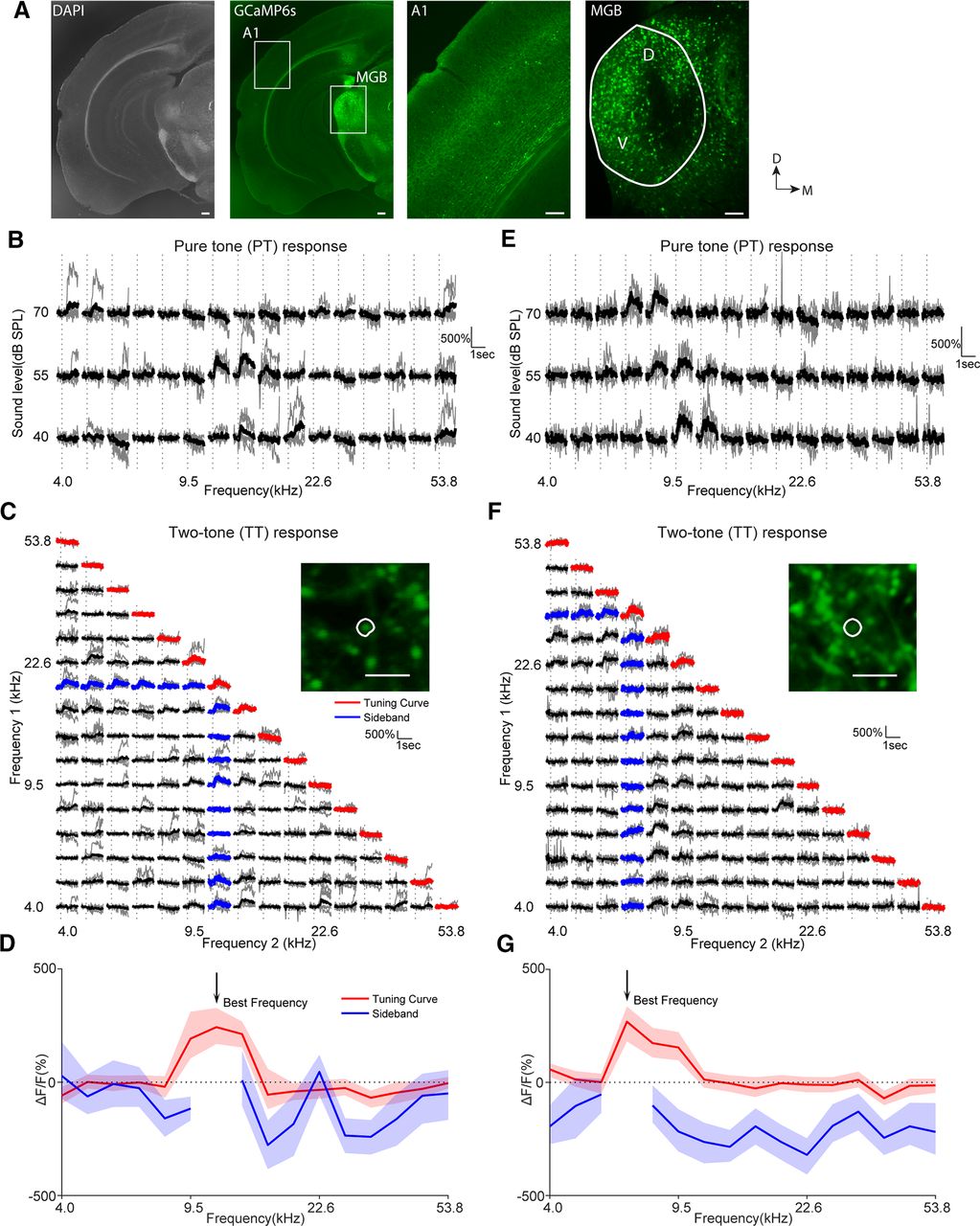
To characterize sideband inhibition in L2/3 of mouse A1, we played both PTs and TT combinations to passively listening awake male and female mice (Fig. 1A). Conventionally, sideband inhibition is inferred by first choosing a reference tone typically at the BF of the neuron in question and then presenting other tones of varying frequencies and sound levels in combination with the chosen tone (Brosch and Schreiner, 1997). By definition, a tone at BF evokes the largest response among frequencies presented across all sound levels. If a tone at BF combined with other tones results in reduced responses, functional inhibition can be inferred at these frequencies (Sutter and Schreiner, 1991). However, this method is ill suited for two-photon imaging, where large neural populations are monitored simultaneously; given the heterogeneity of local tuning (Bandyopadhyay et al., 2010; Rothschild et al., 2010; Winkowski and Kanold, 2013; Bowen et al., 2020), it would be impossible to use the same reference tone for every neuron. Therefore, we designed an alternative approach using a fixed sound level and presenting tones of all possible combinations given the chosen frequency range (3.75 octaves) and density (four tones per octave). This strategy thus resulted in 120 distinct tone pairs given 16 different tones (4–53.8 kHz, logarithmically spaced). We presented two sets of stimuli. The first set of stimuli consisted of the same 16 tones at three sound levels (40/55/70 dB SPL) to construct the FRA. The second set of stimuli consisted of both individual PTs and all 120 tone pairs whose waveforms were linear summations of the PTs. In this second set, the PTs were presented at 60 dB SPL and thus the TTs were 63 dB SPL as they were the linear summation of two different frequencies. Figure 1 shows two examples of responses to the two sets of stimuli in excitatory neurons. Figure 1B shows the responses of an example neuron to PT stimuli. This neuron had a V-shaped FRA with its BF at 19 kHz (Fig. 1D, red curve). Presenting TTs showed that in the presence of a second tone other than 19 kHz, the evoked change in the fluorescence signal (i.e., ΔF/F) was reduced compared with that evoked by the BF alone (Fig. 1C). We thus inferred the inhibitory sideband as frequencies that, when presented together with BF, resulted in a reduction of responses to BF alone. This analysis revealed the presence of sideband inhibition flanking the BF (Fig. 1D, blue curve). Figure 1E–G shows another Thy1 neuron with an I-shaped FRA. This neuron not only showed sideband inhibition, but also showed a facilitative TT effect (Fig. 1F,G, arrows). As our goal is to infer the inhibitory sideband, we focused mainly on the suppressive effect.

Inhibitory sideband can be inferred using TT stimuli combined with two-photon imaging of GCaMP6s across neural populations. Example responses to PT and TT of two Thy1-GCaMP6s neurons within the same field of view and their respective tuning curves and inhibitory sidebands are shown here. A, Experimental paradigm of the current study. Awake mice were passively listening to PT and TT stimuli, while different cell classes in the left A1 were imaged. The location of A1 was determined by performing wide-field imaging. Example wide-field maps are shown on the right. The contour lines of different colors indicate the region of fluorescence increase following the presentations of pure tones of corresponding frequencies. Scale bar, 300 µm. The example two-photon field of views show Thy1-GCaMP6s neurons and viral expression of GCaMP6s and mRuby in PV and SST interneurons. Scale bars, 20 µm. B, Example responses to PT of one Thy1 neuron. The gray traces represent responses in individual trials, and average responses are plotted in black. Vertical dotted lines indicate the onset of the stimulus. The asterisks indicate significant responses determined by nonoverlapping 99.9% confidence intervals of ΔF/F over prestimulus and poststimulus periods. For example, the prestimulus and poststimulus CIs were −17% to 19% and 29% to 84%, respectively, for the stimulus with the red asterisk, and thus this stimulus evoked a significant response. For the stimulus with the red cross, the prestimulus and poststimulus CIs were −19% to 18% and −22% to 11%, respectively, and thus the response was not significant. C, Example responses from the same neuron as in B to TT stimuli. Note that the traces on the diagonal were responses to PTs in the second stimulus set (see Materials and Methods), while off-diagonal traces were responses to TT combinations (inset). The traces with averages plotted in red or blue were used to construct the tuning curve and sideband, respectively in D. D, Tuning curve and inhibitory sideband of the same neuron shown in B and C. The solid lines indicate mean responses, while the shaded regions show 99.9% confidence intervals. For tuning curves, the ΔF/F reflects the percentage of fluorescence change from baseline following the different PTs. For inhibitory sidebands, ΔF/F following the BF tone was subtracted from the ΔF/F following the TT stimuli containing the BF. A significantly negative value suggests a suppression of the response because of the presence of a second tone other than BF. E–G, Same as in B–D but for another Thy1-GCaMP6s neuron with an I-shaped FRA. Note that this neuron showed both TT suppression and facilitation. In F, the arrow points to one example of TT facilitation where PTs presented alone failed to excite this neuron. G, The sideband of this neuron showed mostly suppression except for one frequency (arrow) that evoked facilitation.
We proceeded to record from both excitatory (Thy1-GCaMP6s; Dana et al., 2014) and inhibitory (PV-cre and SST-cre animals with viral expression of GCaMP6s; Fig. 1A) neurons. All mice used in this study were F1 generations from crosses with CBA/CaJ mice to ensure normal hearing throughout adulthood (Frisina et al., 2011). Table 1 lists the basic statistics of responding neurons such as the percentage responding to PTs, to TTs, or to both. We characterized a neuron as responding and analyzed it only if it responded significantly to at least one stimulus (see Materials and Methods). A total of 5576 Thy1 neurons, 1324 PV interneurons, and 1451 SST interneurons passed this criterion, and all subsequent analyses are focused on them. Figure 2 shows example responses from one PV and one SST interneuron, confirming that our approach is applicable to interneurons as well.
Basic response properties across cell types

Inhibitory sidebands can be inferred with TT stimuli in PV and SST interneurons. A, Example FRA of one PV interneuron. The gray traces show individual trials, while the black traces show the trial average. Vertical dotted lines indicate the onset of the stimulus. B, Example responses to TT from the same PV neuron as shown in A. The diagonal responses were to PTs while the off-diagonal responses were to TTs that were the combinations of all PT pairs. C, The tuning curve and inhibitory sideband of the same PV neuron as shown in A and B. The solid lines indicate mean responses, while the shaded regions show 99.9% confidence intervals. D–F, Same as in A–C but for an SST interneuron.
FRA shapes of A1 neurons form cell type-dependent classes
We observed a high degree of variability in the shapes of FRAs of all responding neurons (Fig. 3), similar to recordings in cats (Sutter and Schreiner, 1991; Sutter et al., 1999). We hypothesized that the shape of the FRAs could be linked to properties of sideband inhibition. We thus sought to first classify FRAs based on their shapes. In short, we aligned the FRAs at the geometric center by averaging frequencies weighted by responses across sound levels and performed K-means clustering based on PCA components that kept the 95% of the total variance in the aligned FRA. Figure 4A shows the t-SNE plot of the PCA scores, which embeds high-dimensional data such as the PCA scores for visualization in low-dimensional space, as well as generated labels and their corresponding average FRAs. These unsupervised classification results suggest that there are at least six distinct types of FRAs given the stimulus set in the current study. Intuitively, cluster 1 and cluster 2 corresponded to typical V- and I-shaped FRAs, while the most distinct feature of cluster 3 was its wide tuning at the loudest sound level and sparser responses at lower levels. Clusters 4, 5, and 6 typically only responded to one frequency and sound level combination and thus had the sparsest responses. To further improve the accuracy of the clustering, we manually examined the labels assigned to each cell and corrected misclassifications. Among the total 8351 neurons, 4619 labels were corrected. The final labels were V, I, H, S1, S2, and S3, where H stands for “horizontal” and S stands for “sparse.” Figure 4A shows the average FRAs of the corrected labels. We quantified the variability within each cluster before and after manual correction by computing the interquartile range of the responses across neurons at each aligned frequency. The corrected clusters showed variability mainly within their respective shapes, indicating that the manual classification better retains the consistency of shapes within each cluster (Fig. 4B). We further quantified the proportion of misclassification by calculating for each final manual cluster the compositions of the original K-means result (Fig. 4C), which shows that the misclassification happened majorly among putative V- and I-shaped neurons, while H- and S-type neurons were mostly accurately classified. To further validate the distinctness of the FRA types, we plotted the response profiles either over frequency or over sound level as a function of cell types (Fig. 4D). All FRA types had most of the frequency responses at the center of the FRA except for H type, which had the smallest slope in its cumulative curve over frequency, because of its wide tuning (Fig. 4D, left). The differences between FRA types were more pronounced in the response profile over sound level (Fig. 4D, right). All S types had most of the responses at the sound level to which they were most selective. I types had a rather linear profile, while V and H types showed supralinear profiles because of widening tuning at higher sound levels (Fig. 4D, right). These results suggest that the labels generated by our semiautomatic classification reflect true differences in the selectivity of neurons to both frequency and sound levels.

The FRAs of individual neurons show a large variability. Six different FRAs from Thy1 neurons were plotted to show the variability of FRA shapes across neural populations. In each panel, the image of the neuron was shown in the left top corner with the red line indicating its contour. The white scale bar in the image shows 10 µm. For FRA traces, all horizontal calibration bars indicate 1 s, while vertical calibration bars indicate 300% ΔF/F. All gray traces show individual trials, while the black traces show the trial average. These examples differed in their sparseness of responses as well their selectivity for frequency and sound level. For example, in the second row these neurons responded only to one frequency and sound level combination and thus showed the highest level of sparseness in their FRAs.

Classification of FRA shapes reveals distinct receptive field types. A, Left, t-SNE plot of PCA coefficients of aligned FRAs with data points color coded with their corresponding K-means clusters. Right, Top row, Average aligned FRAs of the six clusters as determined by K-means algorithm. Right, Bottom row, Average aligned FRAs of manual classification based on K-means result. Clusters 1–6 approximately correspond to the color-matched manual classification result in the bottom row. B, The variability within the K-means cluster and that within the manually classified cluster were compared. We quantified the variability at each aligned frequency by computing the interquartile range of response amplitude at the aligned frequency across neurons. The color-matched plots share the same color axis. The manual classification results showed higher variability within their perspective shape (e.g., cluster 1 vs V and cluster 2 vs I). C, To quantify the misclassification, for each final manual label, the proportion of the original K-means cluster is plotted. For example, the first column shows the proportion of the original clusters that constituted the final V-shaped cells (i.e., 19.6% from cluster 1, 44.8% from cluster 2, 19.8% from cluster 3, 2.1% from cluster 4, 7.7% from cluster 5, and 6.1% from cluster 6). Thus, each column has the summation of 1. The most misclassification happened among the putative V- and I-shaped neurons (clusters 1 and 2), while H- and S-type neurons were more accurately assigned. D, The FRA clusters differed in their frequency and sound level response profile. Each line represents the normalized cumulative summation of responses over either frequency (left) or sound level (right). For each cell, the summation was normalized such that the maximum was 1. The shaded regions show 95% confidence intervals. E, The proportion of FRA types within each cell type.
We performed the classification on FRAs of all cell types and further quantified the proportion of FRA types within each cell type (Fig. 4E). For Thy1 neurons, the vast majority of responding neurons belonged to the S types, consistent with the sparse coding of stimuli in sensory cortices (Hromádka et al., 2008). PV and SST neurons had a lower percentage of S-type FRAs than Thy1 neurons. Most notably, both types of interneurons had a higher proportion of H-type FRAs than Thy1 neurons, suggesting a broadening of tuning as the sound level increases. Moreover, PV neurons were the least likely to have I-shaped FRAs, consistent with their broad tuning (Li et al., 2014). These results show a clear cell type-dependent distribution of different FRA types in L2/3 of mouse A1.
Sideband inhibition shows dependencies on FRA shape
We next sought to compare various properties of inhibitory sidebands across both cell types and FRA types. Despite the classification of FRAs, not all neurons responded to the PTs in the TT stimulus set, possibly because of the sparseness of responses or stimulus selectivity for particular frequency and sound level combinations. Table 2 shows the proportion of neurons from which we could infer inhibitory sidebands, and we focused the following analysis on these subsets of neurons. First, we plotted the average tuning curves and inhibitory sidebands for each cell class (Fig. 5A). We then quantified the width of both the tuning curve and the inhibitory sideband. Given that the shape of the tuning curves and sidebands among different neurons could be highly variable, we resorted to a sparseness measure that could be applied to both the tuning curve and inhibitory sideband (see Materials and Method). The fewer frequencies a neuron significantly responded to, the higher the sparseness of the tuning curve, and, given that the sparseness values are bound between 0 and 1, we used 1 – sparseness as the width measure. We found that for all cell types, the width of the inhibitory sidebands was larger than the tuning curve width (Fig. 5B, Table 3). Since inhibitory sidebands are thought to sharpen tuning curves (Li et al., 2014), we hypothesized that the width of the tuning curve and the width of the inhibitory sideband would be negatively correlated. Indeed, a linear fit pooling all cell types and FRA types showed a significant negative slope between the width of tuning curve and that of the inhibitory sideband (Fig. 5C, p = 5.1 × 10⁻¹³), suggesting that a narrower tuning is associated with wider sideband inhibition. These results are consistent with the notion that inhibitory sidebands in cortical neurons contribute to tuning curve sharpening (Li et al., 2014).
Proportion of neurons within each FRA types with sideband inferred

All cell types and FRA types show broader inhibitory sidebands than tuning curves. A, The average tuning curve (solid lines) and inhibitory sideband (dash lines) were plotted as a function of both cell types and FRA types. TC, Tuning curve; SB, sideband. For each cell, the amplitude of the tuning curve and that of the inhibitory sideband were normalized to the amplitude of the BF. Then the normalized tuning curve and inhibitory sideband were aligned at BF to construct both the mean and the confidence interval using bootstrap procedures. B, The widths of the tuning curves and the inhibitory sidebands as measured by 1 – sparseness were plotted as a function of cell types and FRA types. Inhibitory sidebands were considerably larger in width than those of the tuning curves. ***p < 0.001. C, Across all cells, the width of the tuning curve was negatively correlated with the width of the inhibitory sideband. The bar graph shows the inhibitory sideband width binned according to the width of the tuning curve. The dot–dash line shows the linear fit (y = 0.73–0.23x, p = 5.1 × 10⁻¹³).
p Values, Wilcoxon signed-rank test, width of tuning curve versus width of sideband inhibition and effect size measured by Hedges' g
We next investigated the differences of tuning widths across cell types. The widths of the tuning curves were significantly different across cell types (ANOVA, p = 9.9 × 10⁻³⁵) and post hoc multiple-comparisons test revealed that Thy1 neurons had narrower tuning width than both PV and SST neurons (Thy1 vs PV: p = 9.9 × 10⁻¹⁰, effect size measured by Hedges' g = −0.32; Thy1 vs SST: p = 9.6 × 10⁻¹⁰, Hedges' g = −0.48) while PV neurons had narrower tuning width than SST neurons (p = 0.015). However, both Thy1 and PV neurons showed a wider inhibitory sideband than SST neurons (Thy1 vs SST: p = 9.6 × 10⁻¹⁰, Hedges' g = 0.33; PV vs SST: p = 2.4 × 10⁻⁶, Hedges' g = 0.25), while Thy1 and PV neurons did not differ (p = 0.11). Together, these results show that both tuning width and inhibitory sideband width depend on cell types. Specifically, Thy1 neurons had the narrowest tuning width among the three cell types, while the inhibitory sideband width was comparable to PV neurons but wider than SST neurons. Most notably, the width of sidebands was much broader than those of the tuning curves across all cell types and FRA types, suggesting that the highly selective frequency tuning could be because of broad inhibitory synaptic inputs (Li et al., 2014).
The differences between cell types in terms of tuning and sideband widths could be because of their BF. We thus compared the median BF across cell types and found that the median BFs were similar (Fig. 6A). We next compared the tuning BF as a function of both cell types and FRA types (Fig. 6B). Within specific cell types, some differences in BF exist across FRA types. Specifically, we found that Thy1 I-shaped neurons had slightly higher BF median than V-shaped (p = 0.025), S1-shaped (p = 0.031), and S2-shaped (p = 0.037) neurons. The respective 95% CIs of the BF median difference in octaves, computed with a bootstrap procedure, were 0–0.5, −0.25 to 0.5, and 0–0.6250. Since these CIs contain 0, we conclude that the true differences between the BF distributions are relatively small. For PV neurons, only V- and H-shaped neurons showed significantly different BF median (p = 2.0 × 10⁻⁸) and 95% CI of the median difference was −1 to −0.5 octaves. For SST neurons, V-shaped neurons also had a lower BF median than H-shaped neurons (p = 0.0053) with 95% CI of the median difference being −1.25 to −0.25 octaves. Given that these differences existed only in specific pairs of FRA types, they were not likely to significantly impact the results on tuning and sideband width. Similarly, we found that the tuning and sideband width were rather constant within the frequency range of the PT and TT stimuli set, while some differences exist for cells whose BFs were at the low or high end of the frequency range, which is likely because of the lack of data beyond the frequency extremes (Fig. 6C). Together, these results show that across the tonotopic axis of A1, the frequency selectivity of cortical neurons are similar and that they receive a similar amount of sideband inhibition.

BF of tuning curves were not different across cell types. A, Boxplot and cumulative distribution function of tuning BF as a function of cell types. Median BF across different cell types were similar. B, Boxplot and cumulative distribution function (left and mid-column) of tuning BF as a function of both cell types and FRA types. The rightmost column shows the pairwise comparison significance of tuning BF as a function of FRA types. BF difference was only found in between specific FRA subtypes within each cell type. C, The widths of tuning curve and inhibitory sideband were largely similar across tuning BF in all cell types, except for at the low- or high-frequency end, which is likely because of the lack of data beyond the frequency range chosen for this study. n.s., not significant.
Inhibitory sidebands of local populations show a higher degree of heterogeneity than frequency preference
Tonotopy on the mesoscale is a defining characteristic of A1, but on a finer spatial resolution such organization is largely lost as individual excitatory neurons in a local area can have heterogeneous frequency selectivity (Bandyopadhyay et al., 2010; Rothschild et al., 2010; Winkowski and Kanold, 2013; Kanold et al., 2014; Maor et al., 2016; Liu et al., 2019; Bowen et al., 2020). Since we here show the presence of inhibitory sidebands, we investigated whether such heterogeneity exists in the inhibitory sideband of different cell types in a local area. We quantified the heterogeneity of local tuning by computing the IQR of the BF within a radius of 100 µm. A large IQR would indicate a more diversely tuned local populations. Similarly, we defined the BIhF as the frequency evoking the strongest inhibition in the sideband and quantified the IQR of BIhF (Fig. 7). A two-way ANOVA (cell type × BF/BIhF) revealed a significant main effect of cell types on IQR (p = 6.1 × 10−47). Specifically, Thy1 neurons had greater overall heterogeneity than PV neurons (post hoc multiple-comparisons test, p = 9.6 × 10⁻¹⁰, effect size as measured by Hedges' g = 0.6050) and SST neurons (p = 1.1 × 10⁻⁹, Hedges' g = 0.2380), while PV neurons showed less heterogeneity than SST neurons (p = 9.6 × 10⁻¹⁰, Hedges' g = −0.2540). These results are consistent with in vivo patch-clamp recordings showing a higher level of heterogeneity in excitatory than PV neurons (Maor et al., 2016). Second, the main effect of BF versus BIhF was also significant (p = 6.5 × 10−57) with the IQR of BIhF higher than the IQR of BF across cell types (p = 1.0 × 10⁻¹⁰, Hedges' g: Thy1, −0.3488; PV, −0.4971; SST, −0.3379), suggesting that the heterogeneity of inhibitory sidebands was greater than that of tuning of local populations. This heterogeneity of inhibitory sidebands suggests that diverse sources of functional inhibition as an aggregate result in the inhibitory sideband. Last, the interaction term (cell type × BF/BIhF) was also significant (p = 2.8 × 10⁻³). Specifically, the differences between BF and BIhF IQR within Thy1 neurons were smaller than those within PV and SST neurons (ANOVA and multiple-comparisons test; Thy1 vs PV: p = 0.001, Hedges' g = −0.1722; Thy1 vs SST: p = 0.044, Hedges' g = −0.0931). Together, these results suggest that the combined heterogeneity in the tuning and inhibitory sideband of the local populations could further diversify the response of a neuron to spectrally complex stimuli and thus make its responses more selective.

Inhibitory sidebands show more local heterogeneity than tuning curves. A, Cartoon for IQR calculation. The cell in question is represented as the black circle at the center. Cells within a 100 µm radius are plotted. The left and right half of the circle color code the difference of BF and BIhF in octave, respectively, with the center cell. Gray circles represent nonresponding cells. The IQRs are then calculated taking the interquartile range of BF and BIhF Δoctave (oct). B, The heterogeneity of the selectivity of the local tuning and inhibitory sideband was quantified by calculating the IQR of BF or BIhF, respectively. The IQR of BIhF was larger than that of BF across all cell types. ***p < 0.001, n.s., not significant.
The presence of the second tone decorrelates neuronal responses
The differences in the IQR of BF and BIhF suggest that the introduction of the second tone influences neuronal coding of the primary tone on the population level. Thus, to measure this influence we next quantified the signal correlations (SCs) to the primary tone with or without the second tone (Fig. 8A). We performed a two-way ANOVA to determine the dependence of SC on both cell types and the addition of the second tone. The main effect of cell type was significant (p < 0.001) and so was the main effect of adding the second tone (p < 0.001). Specifically, across all cell types the SC of TT was lower compared with that of PT (p = 1.0 × 10⁻¹⁰). Regardless of stimulus type, SCs of Thy1 cells were lower than those of both PV and SST neurons (Thy1 vs PV: p = 9.6 × 10⁻¹⁰, Hedges' g = −0.6534; Thy1 vs SST: p = 9.6 × 10⁻¹⁰, Hedges' g = −0.7917), while SCs of SST neurons were highest among the three cell types (PV vs SST, p = 9.6 × 10⁻¹⁰, Hedges' g = −0.1253). This suggests that PV and SST neurons are more functionally homogeneous than Thy1 neurons, likely because of convergent local input, consistent with results by Maor et al. (2016). In all cell types, SCs of TT were lower compared with SCs of PT (Thy1: p = 2.1 × 10⁻⁸, Hedges' g = 0.036; PV: p = 2.1 × 10⁻⁸, Hedges' g = 0.065; SST: p = 2.1 × 10⁻⁸, Hedges' g = 0.095). To investigate whether the addition of a second tone caused any change to the spatial pattern of neural correlations, we plotted the SCs against the distance of the cell pairs (Fig. 8B). The SCs of PT and TT decreased over the distance in all cell types, and the SCs of TTs were consistently below those of PTs (Fig. 8B), suggesting a network-level decorrelation of neural responses by the addition of the second tone. These results suggest that a spectrally complex stimulus would make neural responses sparser and effectively more selective to spectral features. These results also indicate that TT responses cannot be readily predicted from responses to PTs alone and that the linear and nonlinear frequency interactions in TT responses need to be characterized.

The presence of the second tone decorrelates neuronal responses. A, Violin plot showing the distribution of SCs as a function of both cell types and stimuli (PT vs TT). SCs of TT responses between pairs of neurons were significantly reduced compared with SCs of PT across all cell types. ***p < 0.001. B, Left, SCs as a function of distance, cell types, and stimulus (PT vs TT). SCs of TTs were smaller in value than SCs of PTs across distance. Solid lines correspond to SCs of PTs, while dashed lines correspond to SCs of TT. The shaded regions show the 95% confidence interval. Right, The difference between SCs of TT and PTs as a function of distance and cell types. Shaded regions show 95% confidence intervals.
Nonlinear frequency interactions depend on both cell types and FRA types
Frequency interactions in the auditory system can be linear or nonlinear (Escabi and Schreiner, 2002). Our experimental design allowed us to investigate the degree of nonlinear interactions between frequencies beyond simple TT suppression. Specifically, if a neuron behaves like a linear filter, then its response to the TT stimuli would be the linear summation to the responses to each frequency presented in isolation:  . Any deviation from the linear assumption signals the presence of nonlinear interactions. We quantified the degree of nonlinear interactions across cell types and separated them based on whether the response to the TT stimulus was larger (facilitation) or smaller (suppression) than that predicted by the linear assumption (Fig. 9A). All cell types showed nonlinear effects and significantly more suppression than facilitation (two-way ANOVA, main effect of facilitation vs suppression: Thy1, p = 1.6 × 10−76; PV, p = 1.1 × 10⁻¹³; SST, p = 2.4 × 10⁻³⁵). Across all FRA types, except H type in SST neurons, all other FRA types showed the same dominance of suppressive nonlinear interactions (Wilcoxon rank-sum test; Table 4, p values and effect sizes), which suggests that the degree of nonlinear interactions could further depend on specific cell type and FRA type combinations. This analysis pooled the degrees of facilitation and suppression across cells and thus reflected the properties on a population basis. To investigate the bias of facilitation and suppression of individual cells, we calculated an SFI, which had values between −1 and 1, with 1 indicating only suppressive interactions and −1 indicating only facilitative interactions. The cumulative distributions of SFIs are shown in Figure 9B. For Thy1 cells, V-, I-, and H-type neurons had the most bias toward suppression while SFI distributions among all S types were not significantly different from each other (Fig. 9B). While V- and I-type neurons had the same SFI distribution, both were higher than that of H-type neurons (V vs H: p = 2.1 × 10⁻⁸, Hedges' g = 0.5018; I vs H: p = 0.001, Hedges' g = 0.3081), suggesting that a broader tuning width was associated with a lesser degree of suppressive frequency interactions. For PV neurons, SFI values were smaller in H-type neurons than in V-type neurons (p = 0.011, Hedges' g = 0.3451). For SST neurons, SFI values were also smaller in H-type neurons than in both V- and I-type neurons (V vs H: p = 3.4 × 10⁻⁵, Hedges' g = 0.4671; I vs H: p = 4.4 × 10⁻⁵, Hedges' g = 0.5799). Therefore, the shape of FRAs could serve as an indicator of the degree of nonlinear interactions and thus delineates functionally separate classes of cells. Specifically, the results above suggest that H-type neurons might be more involved in integrating energy over frequency bands while V- and I-type neurons serve as differentiators of the frequency content.

Nonlinear frequency interactions show prominent suppression among all cell types while the relative facilitation/suppression strength depends on specific cell/FRA type combination. A, The amplitude of facilitative and suppressive nonlinear frequency interactions as a function of FRA types and cell types. In all cell types, the average suppressive interactions were larger in amplitude than facilitative interactions. *p < 0.05. **p < 0.01. ***p < 0.001. B, Top row, SFI (see Materials and Methods) as a function of FRA types and cell types. SFI measures the bias of suppressive or facilitative interactions within individual cells. 1 indicates purely suppressive interactions, while −1 indicates purely facilitative interactions. Bottom row, matrices showing p values of pairwise comparisons among different FRA types within each cell types.
Wilcoxon rank-sum test, p values, and Hedges' g, facilitation versus suppression across cell type and FRA types
Nonlinear frequency interactions as a function of onset and offset response
Our previous study demonstrated that dynamic sound features such as sound onset and offset are processed in parallel processing pathways in the auditory cortex (Liu et al., 2019). Thus, we sought to investigate whether these two pathways might also process spectral information differently and whether differences exist between these pathways in terms of the degree of nonlinear frequency interactions. We first quantified the latency of the cellular responses to identify onset and offset neurons (Fig. 10A). We labeled neurons as either onset or offset neuron (see Materials and Methods) since they largely consisted of separate groups of neurons (Liu et al., 2019). The majority of neurons were onset neurons across cell types and FRA types (Fig. 10B). The lower fraction of offset neurons compared with prior studies (Liu et al., 2019) is likely because of shorter stimulus duration (100 ms vs 2 s) and intertrial intervals (1.5 vs 5–5.5 s). We next compared the amplitude of facilitative or suppressive interactions between onset and offset neurons on a population basis (Fig. 10C). In Thy1 neurons, offset V-, I-, H-, and S1-type neurons had larger facilitative interactions than onset neurons of the same FRA type (Fig. 10C; Wilcoxon rank-sum test; V: p = 2.6 × 10⁻⁷, Hedges' g = −0.93; I: p = 0.022, Hedges' g = −0.50; H: p = 1.5 × 10⁻⁵, Hedges' g = −0.59; S1: p = 7.8 × 10⁻³, Hedges' g = −0.32). In contrast, only H-type neurons showed larger suppressive interactions for offset neurons (Wilcoxon rank-sum test, p = 3.9 × 10⁻⁵, Hedges' g = −0.82). PV neurons generally showed the same degree of facilitative and suppressive interactions across onset and offset neurons, except that PV H-type offset neurons showed larger facilitative interactions than corresponding onset neurons (Wilcoxon rank-sum test, p = 0.003, Hedges' g = −0.42), while PV S1 offset neurons showed slightly smaller facilitative interactions (Wilcoxon rank-sum test, p = 0.026, Hedges' g = 0.17). SST neurons also showed a similar degree of nonlinear interactions across onset and offset neurons except that V- and H-type offset neurons had larger facilitative interactions than V- and H-onset neurons (Wilcoxon rank-sum test; V: p = 2.2 × 10⁻⁷, Hedges' g = −0.59; H: p = 1.5 × 10⁻⁵, Hedges' g = −0.50), which is similar to that seen in Thy1 neurons. These results show that a subset of offset neurons tended to have larger nonlinear facilitative interactions than their onset counterparts. This suggests that the offset pathway not only conveys temporal information, but also tends to integrate spectral information supralinearly to a larger degree than onset neurons, and thus could be more suited to encode the general energy level in the stimulus.

Nonlinear frequency interactions as a function of response timing. A, The average traces of onset and offset responses pooled from all responding neurons. Dotted vertical lines mark the onset and offset of the stimulus, respectively. B, Proportion of onset and offset neurons as a function of cell type and FRA types. C, Nonlinear frequency interactions as a function of response timing, FRA types, and cell types. A subset of offset neurons showed a higher degree of facilitative interactions than their onset counterparts. *p < 0.05; **p < 0.01; ***p < 0.001.
MGB responses exhibit sideband inhibition
A1 neurons receive feedforward input from the auditory thalamus or MGB, and it is thus possible that the sideband inhibition seen in cortical neurons is partially inherited from thalamocortical input. To investigate this question, we injected AAV.CaMKII.GCaMP6s.WPRE.SV40 into the MGB and imaged MGB terminals in A1 (Liu et al., 2019; n = 3 mice, 17 FOVs; Fig. 11A). Our labeling of MGB neurons included ventral and dorsal division, and thus the imaged boutons likely consisted of both first- and second-order thalamic inputs (Fig. 11A). The MGB terminals had denser labeling in L1 and L4, consistent with previous findings (Vasquez-Lopez et al., 2017). We imaged at a depth of 117 ± 19.5 µm, and, as L1 and L3b/4 MGB boutons show similar tuning (Vasquez-Lopez et al., 2017), the PT and TT responses were not likely affected by this choice of depth. Among all putative boutons recorded, 47.1 ± 12.2% responded to at least one PT stimulus, 54.2 ± 12.8% responded to at least one TT stimulus, 40.3 ± 12.6% responded to both PT and TT stimuli. Figure 11B–G shows two example boutons with respective FRAs and responses to TT and the corresponding sideband inhibition. These results show that sideband inhibition exists in thalamocortical input. Similar to our cellular data, we also observed considerable variability in the shapes of the MGB terminal FRAs, and, following the same approach as above, we classified the FRA shapes (Fig. 12A). However, the MGB clusters were not as separated as seen in cellular data (Fig. 2B), which could be because of the limited signal-to-noise ratio of bouton imaging that resulted in failed detection of smaller responses. Nevertheless, the average FRAs of the clusters resembled those seen in cellular data (Fig. 12A). Specifically, cluster 1 approximately corresponded to a combination of narrow V and I shapes, while cluster 2 corresponded to the putative H shape. The average FRA of cluster 3 suggests a broad tuning, and yet the average tuning curve suggests otherwise (Fig. 12A,B). Thus, this cluster has a large within-cluster variation and might not have a well defined FRA shape. We speculate that this cluster might represent responses from a nonlemniscal pathway such as dorsal MGB (dMGB), as our injections were not restricted to particular divisions of MGB (Fig. 12A) and dMGB responses are weakly tuned (Vasquez-Lopez et al., 2017). Clusters 4 and 5 likely corresponded to the S1 shape, and cluster 6 corresponded to the S2 shape. However, S3 type was not recovered in MGB data. These results show that the responses of individual MGB boutons to tones also showed large FRA variability. We then proceeded to quantify the widths of both tuning curves and inhibitory sidebands in these clusters. On average, all clusters showed much broader inhibitory sidebands than tuning curves (Fig. 12B,C; Wilcoxon sign-rank test; cluster 1: p = 8.3 × 10−96, Hedges' g = −3.20; cluster 2: p = 2.8 × 10−105, Hedges' g = −3.97; cluster 3: p = 2.7 × 10−277, Hedges' g = −5.49; cluster 4, p = 4.7 × 10−85, Hedges' g = −4.79; cluster 5: p = 8.1 × 10−129, Hedges' g = −5.66; cluster 6: p = 1.7 × 10−104, Hedges' g = −5.36), also similar to our cellular data (Fig. 5B). These data suggest that MGB input might contribute to sideband structures seen in cortical neurons. Finally, we compared the sparseness of the tuning width and inhibitory sideband of MGB terminals with those of cellular data (Fig. 12D). We found that MGB terminals showed significantly narrower tuning than all cortical cell types examined (ANOVA and multiple-comparisons test; MGB vs Thy1: p = 7.8 × 10⁻⁴, Hedges' g = −0.11; MGB vs PV: p = 3.8 × 10⁻⁹, Hedges' g = −0.49; MGB vs SST: p = 3.8 × 10⁻⁹, Hedges' g = −0.67). In contrast, MGB terminals showed a broader inhibitory sideband than those of cortical neurons (ANOVA and multiple-comparisons test; MGB vs Thy1: p = 0.0097, Hedges' g = 0.086; MGB vs PV: p = 3.5 × 10⁻⁴, Hedges' g = 0.17; MGB vs SST: p = 3.8 × 10⁻⁹, Hedges' g = 0.42). These results are consistent with narrower tuning of MGB neurons relative to A1 neurons in the awake marmoset (Bartlett et al., 2011). Together, MGB terminals showed more pronounced sideband inhibition than the three cortical neuron types examined, which suggests that the narrowly tuned MGB feedforward input serves as the backbone for cortical inhibitory sidebands and that the wider tuning of cortical neurons reflect the differential patterns of the convergence of connectivity onto different types of cortical neurons by both feedforward thalamocortical and intracortical input (Fig. 12E).
MGB terminals show inhibitory sideband structures. A, Brain slice showing GCaMP6s expression in MGB and MGB terminals in A1. Left two images show DAPI staining and GCaMP6s epifluorescence at low magnification (2×). Scale bars, 200 µm. Right two images show high magnification (10×) views of outlined areas. Scale bars, 100 µm. Axon terminal GCaMP6s expressions can be seen in L1 and L4. B–G, Two examples of the response of MGB boutons to PT and TT are shown. B, FRA of one example bouton. C, Example responses to TT stimuli. Gray traces represent individual trials in both B and C. The blue and red average traces indicate the responses used to construct the tuning curve and the inhibitory sideband in D. The inset shows the image of the bouton, with the white contour line outlining the ROI mask. Scale bar, 5 µm. D, The tuning curve and inhibitory sideband of the bouton. E–G, Same as in A–C but for another bouton.

MGB terminals show narrow tuning and prominent sideband inhibition. A, t-SNE plot showing the distribution of center-aligned FRAs of MGB terminal FRAs. The colors indicate the clusters from the K-means algorithm. Right, Average center-aligned FRAs of the K-means clusters. B, Average tuning curves and inhibitory sidebands of clustered MGB terminals. All clusters showed narrow tuning and broad inhibitory sidebands. C, Bar plot showing the width of tuning and inhibitory sideband as a function of clusters. In all clusters, the inhibitory sidebands were much broader than tuning curves. ***p < 0.001. D, Bar plot comparing tuning width and sideband width among different cortical cell types and MGB terminals. MGB terminals show narrower tuning than cortical neurons while having broader inhibitory sidebands. E, Cartoon showing a model for cortical tuning and sideband inhibition. The cortical neurons partially inherit inhibitory sideband structures from the thalamocortical MGB input, and the width of tuning and sideband inhibition reflect the differential convergence of input within intracortical circuits (i.e., from neurons tuned to other frequencies; gray triangles and connections). Triangles represent Thy1 neurons, while white and gray circles represent PV and SST neurons, respectively.
Discussion
We used a variant of the TT paradigm suitable for two-photon imaging and characterized the sideband inhibition of excitatory neurons (Thy1) and two classes of inhibitory neurons (PV and SST) in A1. Imaged cells clustered into subtypes based on the shapes of FRA and the degree of sideband inhibition and nonlinear frequency interactions. This suggests that sound information in A1 is locally processed in distinct neuronal population with varying degrees of complex integration of spectral information. The wide inhibitory sidebands suggest a tight control of frequency tuning by inhibition. The mostly suppressive nonlinear frequency interactions also suggest inhibition as a key modulator of spectral integration and thus plasticity. Moreover, we found that cells showing onset and offset preferences showed different spectral integration, suggesting that these cells form different neuronal circuits. Finally, we found that MGB terminals show inhibitory sidebands, suggesting that feedforward inputs contribute to cortical sideband inhibition.
A1 neurons formed six distinct clusters based on their FRA. These clusters differed in their apparent shapes, namely in their frequency and sound level selectivity. In excitatory Thy1 neurons, the majority (∼75%) of the responding cells belonged to the S types where their FRAs were patchy and sparse, while ∼25% of the responding cells belonged to V, I, or H types. With an overall response rate of ∼35%, this suggests that ∼9% all excitatory cells have “classic” V-shaped FRAs, consistent with a sparse coding regime with only ∼5% of auditory responsive neurons (Hromádka et al., 2008). Notably, our results suggest a negative correlation between tuning and inhibitory sideband width. Together, these results suggest that functional inhibition controls the sparseness and tuning width of responses in A1, consistent with the contribution of PV interneurons to sparse coding of local pyramidal cells (Liang et al., 2019). The wide range of inhibitory sidebands also implies that adjusting inhibitory sidebands could be a potential mechanism to rapidly change cellular tuning during task performance (Fritz et al., 2010; Winkowski et al., 2013; Francis et al., 2018).
Pyramidal neurons in L2/3 of mouse A1 can be classified into five groups based on their cellular location and functional excitatory and inhibitory connectivity pattern (Meng et al., 2017), suggesting that these cells would likely show differential tuning properties. Here the FRAs of L2/3 neurons could be classified into six different groups, and we speculate that these clusters correspond to cells with differential connectivity patterns. L2 neurons are more likely to have recurrent lateral connections, while deeper L3 neurons show more feedforward L4 input, which is correlated with a broader tuning at more superficial layers (Meng et al., 2017). Within our classification, H-type neurons had the broadest tuning at 70 dB SPL, and PV and SST neurons are more likely to include such types of neurons. SST neurons in L3 of mouse A1 mostly receive excitatory input from superficial layers (Oviedo, 2017), suggesting that local connectivity patterns could bias tuning selectivity in vivo.
Our results suggest that the sideband inhibition observed in cortical neurons originates both from MGB terminals and intracortical sources. The source of cortical sideband inhibition in A1 has been attributed either to PV neurons (Li et al., 2014) or to SST neurons (Kato et al., 2017; Lakunina et al., 2020). One confounding factor is that these prior studies differed in their methods for inferring inhibitory sidebands. Li et al. (2014) used the classic TT paradigm with one tone (100 ms in duration) of varying frequency and sound levels and the other held constant at the characteristic frequency of the cell. In contrast, Kato et al. (2017) used 1 s tones and inferred sideband inhibition from frequencies that resulted in below-baseline fluorescence deflection, which could underestimate inhibition. Last, Lakunina et al. (2020) used increasing bandwidth of bandpassed noise (1 s duration) centered at the BF of the cell and inferred the sideband through suppression of the firing rate. The differences in stimulus duration can potentially bias the relative contribution of PV and SST neurons. PV neurons receive feedforward input as a part of the “driver” pathway that typically exhibits synaptic depression (Lee and Sherman, 2010). In addition, inhibitory synapses onto pyramidal cells also show strong synaptic depression (Bridi et al., 2020). Together, these two mechanisms suggest that the inhibition from PV neurons onto pyramidal neurons weakens as stimulus duration is prolonged. In contrast, it is likely that SST neurons are specialized in sustained inhibition during long stimuli. Inhibitory neurons show within-group cooperativity and cross-group inhibition (Karnani et al., 2016), and our previous work showed that SST and PV neurons show activity of the opposite sign during prolonged stimuli (Liu et al., 2019). These results suggest that SST neurons mediate sustained inhibition to both local excitatory neurons and PV neurons. In contrast, PV neurons might be more involved in mediating disynaptic feedforward inhibition at the onset of the sensory stimuli (Li et al., 2014). Nevertheless, the relative contributions of PV and SST toward sideband inhibition as a function of the duration of the sensory stimuli remain unclear.
SST neurons provide dense and nonspecific inhibition onto local pyramidal cells (Fino and Yuste, 2011), and they have high connection probability with local pyramidal neurons (Levy and Reyes, 2012). Thus, if SST neurons play a major role in shaping inhibitory sidebands, neighboring pyramidal cells should have similar inhibitory sidebands. However, our IQR analysis of BIhF shows a higher degree of sideband heterogeneity than local frequency tuning. Therefore, our results suggest that sideband inhibition might not originate from a uniform source but reflects multiple sources. Given that we find prominent inhibitory sidebands in MGB terminal responses, our result suggests that inhibitory sidebands arise from the complex interplay between feedforward input from the thalamus and the processing by local microcircuits. This view is consistent with a linear amplification of thalamocortical inputs by L4 (Li et al., 2013), which would include both excitation and disynaptic inhibition. The tuning of MGB terminals was narrower than the three types of cortical neurons, consistent with results in the marmoset (Bartlett et al., 2011). Thus, it is likely that thalamocortical inputs contribute significantly to the observed cellular inhibitory sidebands. Moreover, as sideband inhibition originates from the auditory periphery (Ruggero et al., 1992) and can be observed at other stages in the ascending auditory pathway (Konrad-Martin et al., 1998; Jen et al., 2002), we consider the inhibition seen in A1 as functionally diverse with aspects partially generated de novo in A1.
The relative contribution of MGB and intracortical inhibitory sources likely varies by relative frequency to BF. PV and SST neurons likely contribute to inhibitory sideband far from BF. Our data show that PV and SST neurons had higher SCs over distances than Thy1 neurons, suggesting that these interneurons are suited to convey inhibition of frequencies far from the characteristic frequency. In addition, Natan et al. (2015) found no firing rate change to BF when either PV or SST neurons were silenced, while responses to nonpreferred frequencies were slightly disinhibited. In contrast, silencing PV neurons increased the evoked firing rate yet produced no change in tuning width, while silencing SST neurons increased tuning width, but this effect was because of increased firing rate in response to spectral content far from BF (Lakunina et al., 2020). However, these results cannot explain the sideband structure close to BF that we observed in the current study. Such inhibition close to BF could result from feedforward thalamocortical or L4 input. Thus, PV and SST neurons might serve to temporally truncate responses to pyramidal neurons. In A1 L4, the intracortcal connections are thought to selectively amplify EPSCs evoked by frequencies close to BF as cotuned neurons tend to be interconnected (Liu et al., 2007). This circuit could also amplify the TT suppression close to BF. Specifically, as responses of TT and PT close to BF are amplified, their differences are effectively amplified as well, leading to a greater suppressive effect. Therefore, we speculate that feedforward inputs contribute more strongly to sideband inhibition for frequencies close to BF.
We have shown here that the introduction of the second tone decreases neural correlations between cell pairs, which suggests that more spectral complex stimuli result in changes in population encoding. This potentially resulted from prominent suppressive nonlinear interactions between frequency components within the TT stimuli. Nevertheless, facilitative interactions do exist, and the relative strength of suppression versus facilitation depends on specific FRA types. Typically, V- and I-type neurons are most biased toward suppression, while H-type neurons show less such bias because of larger facilitative interactions. This is consistent with findings that L2/3 neurons of mouse A1 consist of subtypes that differentially integrate spectral information (Li et al., 2019). V- and I-type neurons behave similarly to bandpass filters, while H-type neurons behave as integrators of spectral energy. We speculate that these two types of processing could be more relevant to differentiation and detection of sound, respectively. Across cell types, Thy1 neurons showed larger nonlinear interactions overall than PV and SST neurons. However, a possible confound is that evoked fluorescence (ΔF/F) responses could potentially be smaller in PV and SST neurons because of higher baseline fluorescence levels. As the suppressive effect of TT cannot exceed the responses to PT, the detectable nonlinear interactions were bounded by the ΔF/F evoked by PTs.
We found that both onset and offset responding neurons show nonlinear frequency interactions in their responses to TT stimuli. Notably, in some subtypes of neurons (e.g., Thy1 H type), offset neurons show greater nonlinear interactions. To our knowledge, this is the first time such a phenomenon has been shown, suggesting that the pathway conveying offset information in mouse A1 might be engaged differently in integrating sound information and might consist of different neuronal circuits. Our previous study suggested that timing information is relayed from thalamus and is further refined in cortical microcircuits (Liu et al., 2019). Our current result suggests that this pathway is also suited to convey complex spectral interactions, but it is unclear whether the same cortical mechanisms involving PV and SST neurons contributing to spectral interactions are responsible for the same interactions in offset responses.
In summary, our modified TT paradigm has allowed us to reveal inhibitory sideband and nonlinear frequency interactions of large populations of neurons. Neurons form subclasses based on the shape of FRAs and the differential degree of nonlinear frequency interactions. Moreover, spectrally complex stimuli like TT resulted in decorrelation of neural responses, suggesting a sparse and more selective encoding of sound with rich spectral content. The local heterogeneity of sideband inhibition suggests that these sidebands might reflect integration of multiple sources. Last, we found prominent sideband inhibition in MGB terminals. Together, our results show that cellular tuning properties in a local region might not result from a uniform set of sources but from feedforward input with existing sideband structures arising from subcortical processing stages and further diverse contributions from local cortical inhibitory sources.
Footnotes
This work was supported by National Institutes of Health | National Institute on Deafness and Other Communication Disorders Grant R01-DC-009607 (to P.O.K.).
The authors declare no competing financial interests.
- Correspondence should be addressed to Patrick O. Kanold at pkanold{at}jhu.edu


