Summary
We describe a novel methodology for creating naturalistic 3-D objects and object categories with precisely defined feature variations. We use simulations of the biological processes of morphogenesis and phylogenesis to create novel, naturalistic virtual 3-D objects and object categories that can then be rendered as visual images or haptic objects.
Abstract
In order to quantitatively study object perception, be it perception by biological systems or by machines, one needs to create objects and object categories with precisely definable, preferably naturalistic, properties1. Furthermore, for studies on perceptual learning, it is useful to create novel objects and object categories (or object classes) with such properties2.
Many innovative and useful methods currently exist for creating novel objects and object categories3-6 (also see refs. 7,8). However, generally speaking, the existing methods have three broad types of shortcomings.
First, shape variations are generally imposed by the experimenter5,9,10, and may therefore be different from the variability in natural categories, and optimized for a particular recognition algorithm. It would be desirable to have the variations arise independently of the externally imposed constraints.
Second, the existing methods have difficulty capturing the shape complexity of natural objects11-13. If the goal is to study natural object perception, it is desirable for objects and object categories to be naturalistic, so as to avoid possible confounds and special cases.
Third, it is generally hard to quantitatively measure the available information in the stimuli created by conventional methods. It would be desirable to create objects and object categories where the available information can be precisely measured and, where necessary, systematically manipulated (or 'tuned'). This allows one to formulate the underlying object recognition tasks in quantitative terms.
Here we describe a set of algorithms, or methods, that meet all three of the above criteria. Virtual morphogenesis (VM) creates novel, naturalistic virtual 3-D objects called 'digital embryos' by simulating the biological process of embryogenesis14. Virtual phylogenesis (VP) creates novel, naturalistic object categories by simulating the evolutionary process of natural selection9,12,13. Objects and object categories created by these simulations can be further manipulated by various morphing methods to generate systematic variations of shape characteristics15,16. The VP and morphing methods can also be applied, in principle, to novel virtual objects other than digital embryos, or to virtual versions of real-world objects9,13. Virtual objects created in this fashion can be rendered as visual images using a conventional graphical toolkit, with desired manipulations of surface texture, illumination, size, viewpoint and background. The virtual objects can also be 'printed' as haptic objects using a conventional 3-D prototyper.
We also describe some implementations of these computational algorithms to help illustrate the potential utility of the algorithms. It is important to distinguish the algorithms from their implementations. The implementations are demonstrations offered solely as a 'proof of principle' of the underlying algorithms. It is important to note that, in general, an implementation of a computational algorithm often has limitations that the algorithm itself does not have.
Together, these methods represent a set of powerful and flexible tools for studying object recognition and perceptual learning by biological and computational systems alike. With appropriate extensions, these methods may also prove useful in the study of morphogenesis and phylogenesis.
Protocol
1. Creating Naturalistic Virtual 3-D Objects using VM
- To create digital embryos, use the Digital Embryo Workshop (DEW; see Table 1). Each run generates a single embryo14, the shape of which is unique to a given set of settings (or 'genotype') used for the given run (Figure 1). The 'cells' of the embryo are represented as triangles14.
- Run the program as many times as needed to generate the desired number of embryos.
- If more complex shapes are desired, increase the number of growth cycles, i.e. the number of times the cells of the embryo will divide. Note that this will also slow down the program. If it is necessary to create virtual objects other than digital embryos, use commercially available 3-D modeling tools or obtain virtual objects from commercial vendors (Table 1).
- It is generally advisable to save the virtual objects in a commonly used file format, such as OBJ, so that the objects can be readily imported into a commercial 3-D modeling toolkit. To this end, the DEW writes objects in OBJ format by default.
- Visual stimuli can be generated using one or more digital embryos using a 3-D modeling and rendering environment (Table 1). Use standard graphical operations such as varying the orientation, size, lighting, surface texture and background to create the desired stimuli (see Figure 2).
2. Creating Naturalistic Object Categories using VP
- To generate object categories, generate descendants (or 'children') of the given ancestor (or 'parent') object using a desired combination of the processes in Step 1.1 above (Figure 3)9,10,12,13.
- Some methods described below for creating smooth shape variations, such as morphing or principal components (see Steps 3 and 4 below), work better if all the input objects have the same number of cells and if there is one-to-one correspondence among the vertices of the objects. For creating such objects, use only those VM processes that will not change the number of cells and will preserve the one-to-one correspondence of vertices among the objects (see, e.g., generations G2 to G3 in Figure 3). For instance, cell division and programmed cell death alter the number of cells, and make it much harder (although not impossible17,18) to determine one-to-one correspondence between the vertices of a given pair of objects.
Note that the processes that alter the number of cells in a given object also alter its shape complexity. In general, the greater the number of cells, the greater the shape complexity of the object and smoother its surface. - If necessary, virtual objects other than digital embryos can be used as inputs to VP (Figure 4).
- Some methods described below for creating smooth shape variations, such as morphing or principal components (see Steps 3 and 4 below), work better if all the input objects have the same number of cells and if there is one-to-one correspondence among the vertices of the objects. For creating such objects, use only those VM processes that will not change the number of cells and will preserve the one-to-one correspondence of vertices among the objects (see, e.g., generations G2 to G3 in Figure 3). For instance, cell division and programmed cell death alter the number of cells, and make it much harder (although not impossible17,18) to determine one-to-one correspondence between the vertices of a given pair of objects.
- The objects within a given category can be further selected so as to achieve a given distribution of features19. For instance, one can selectively eliminate mid-sized objects from a given category in order to generate a bimodal distribution of object size.
- There is no single method that is universally optimal for measuring the available shape information for all categories, nor is there a single method that is optimal for categorizing all objects20-22. Thus, the experimentor must choose these methods based on the categories and computational goals at hand20-22. Step 4 describes a commonly used method for manipulating various aspects of available shape information.
- The similarity between a given pair of categories can be objectively measured using available phylogenetic methods23,24. For instance, the vertical (or 'evolutionary') distance between a given pair of categories, as measured by hierarchical clustering methods in the R statistical toolkit, is an objective measure of category similarity25,26.
3. Additional Methods of Creating Shape Variation: Digital Morphing
- Given any pair of objects so that each vertex of one object corresponds to exactly one vertex of the other object (i.e., objects with one-to-one correspondence between vertices), morphing is straightforward17,18,27-29: In this case, smooth variations (or 'morphs') between the two objects are produced by smoothly interpolating between the corresponding vertices and normals (Figure 5). Depending on the pair of objects chosen, morphing will result in new categories or additional children within a category.
- The objects shown in Figure 5 were created using linear morphing27-29. The objects can be morphed (or warped) by a vast array of other available deformation techniques17,18.
- To create a desired distribution of morphed shapes, choose the interpolation points accordingly.
4. Additional Methods of Creating Shape Variation: Principal Components
- In order to use principal components to generate shape variations, one needs to first determine the principal components15. Principal components are specific to the given set of objects used for determining them26. For good results, use at least 30 objects with one-to-one correspondence between vertices26.
- Generate an average object from a desired set of n input objects, by separately averaging the coordinates and the normal of each vertex across all objects. Thus, the x coordinate of a given vertex k of should be the average of the x coordinates of vertex k of all n objects, and so forth.
- Use the Matlab function princomp to determine principal components of the n objects. This will generate n-1 non-zero eigenvectors, along with the corresponding n-1 eigenvalues26.
- To generate a new object Aj from a given principal component Pi , multiply Pi by the corresponding eigenvalue λi and a desired weight wj and add to the average object:
Aj= +wjλiPi - Each unique wj will generate a unique object. By smoothly varying w, one can create smooth shape variations along a given principal component.
- To create shape variations along an independent shape dimension, repeat step 4.4 using a different principal component.
- To create a desired distribution of shapes along a given principal component, use the desired distribution of w.
- To create a multi-dimensional grid of shapes, use a set of weights for each of several principal components:


5. Creating Haptic Versions of 3-D Objects
- 'Print-out' 3-D objects using a 3-D prototyper (or 3-D 'printer'). If necessary, adjust the object's size and smooth the object's surface prior to printing.
6. An Exemplar Application: Bayesian Inference of Image Category
- An important task in visual processing is inferring the category to which a given observed object belongs. Although the exact mechanism of this inference is unknown, there is both computational and physiological evidence 9,12,13,30-32 that it involves using the information about known features of the object in the given image to infer the category of the object. Here, we will illustrate how this inferential process may work in a Bayesian framework, and how digital embryos may be useful for research in this area.
- For simplicity, we will assume that the categorization task is binary and involves distinguishing category K from category L (Figure 3). Let C be the category variable. We will infer that C = K or C = L according to whether the observed image I belongs to category K or L. A typical approach to categorization involves:
- Computing the probability that the category is K given the information in the image, denoted p(C = K |I);
- Computing the probability that the category is L given the information in the image, denoted p(C = L | I); and
- Picking the category with the higher probability.
- Next, we will assume for simplicity that there is exactly one binary feature F. This feature may be either present in the image (denoted F = 1) or absent from the image (denoted F = 0). This example will use the 'informative fragment' feature shown in Figure 8. Informative fragments were first described by Ullman and colleagues33. In the present case, we will use the image template shown in Figure 8 as the feature, and a threshold value of 0.69. To determine whether this feature is present in a given image (say, the rightmost image in row G3 in Figure 3), we will use the following steps:
- Slide this template over all possible locations in the image and compute, at each location, the absolute value of normalized cross-correlation between the template and the underlying sub-image.
- Select the image location with the highest value (0.60 in the present case).
- If this value is above the threshold, conclude that the feature is present; otherwise, conclude that it is absent. In our case, since the highest correlation 0.60 is below the threshold of 0.69, we conclude that the feature is absent in this image.
- The rationale of using such features, and the mechanisms of selecting features and determining their thresholds are beyond the scope of this report, but are described in detail in refs. 33, 30.
- Within the framework of feature-based inference, we assume that all the information the observer extracts from the image is contained in the value of this feature, i. e., that p(C | I) = p(C | F).
Therefore, the task becomes that of determining the value of F in the given image (present or absent), computing p(C = K | F) and p(C = L | F) for that value F, and selecting the category with the higher probability. - In the Bayesian framework,

Therefore,

and

Note that the denominator in the two equations is the same. Therefore, to compare p(C = K | F) and p(C = L | F), it is not necessary to compute the denominator; rather, it is sufficient to compute the quantities
p(C=K|F) ∝ p(C=K)p(F|C=K)
and
p(C=L|F) ∝ p(C=L)p(F|C=L)
These are sometimes called 'unnormalized probabilities'. The term p(C) is called 'prior', and the term p(F | C) is called 'likelihood'.
- For simplicity, we will assume a 'flat' prior: p(C = K) = p(C = L) = 0.5.
- The task is now to compute p(F|C), the probability of a given feature value in an image of a given category C.
- We will use the six images of category L (Figure 3) as an example to compute p(F = 1|C = L), the probability that the feature is present in an image of category L.
- To compute p(F = 1|C = L), first take all the training images that belong to L. Again, these are shown in Figure 3.
- For each image, determine whether the feature value is 1 (present) or 0 (absent), as described in (6.3.1)-(6.3.3). In our case, for the six images in Figure 3, the values are: [0, 0, 1, 0, 1, 0].
- Compute the fraction of images in which the feature value is 1. In our case, it is 2/6 = 0.33.
- Therefore, p(F = 1|C = L) = 0.33. Note that to obtain accurate estimates, one should use at least 30 images per class.
- In a similar manner, we can compute that p(F = 0|C = L) = 0.67, p(F = 1|C = K) = 0.83, p(F = 0|C = K) = 0.17.
- Given these values, inference can be performed. Assume that we are given a new image (Figure 9), and the task is to determine its category label. This is performed as follows:
- We determine whether the feature F is present in the image, as described in (6.3.1)-(6.3.3). In our case, the feature is present, so F = 1.
- Using equations (1) and (2), and the values computed in (6.7.5)-(6.7.6), we can calculate that p(C = K | F = 1) = 0.42 and p(C = L | F = 1) = 0.17.
- Given this information, it is rational to conclude that the image is from category K, with relatively low confidence.
- It could be interesting and useful to test such an approach in a biological system (say, psychophysically). In this case, behavioral predictions could be made and compared against the computational results such as those obtained in (6.8.2). To make accurate predictions, good estimates of p(F |C) are necessary. Such estimates, however, may be difficult to obtain for familiar objects. The reason is that a subject's estimate of p(F |C) is not observable directly, and it is extremely difficult to compute it since the subject's prior exposure to natural images is uncontrollable and unknown. In contrast, if digital embryos are used for the experiments, then it is possible to precisely control which embryos and embryo categories the subject is exposed to. This makes it easy to compute the quantities of interest from exactly the same data the subject was exposed to. The fact that embryos' appearance is naturalistic is helpful, since it makes it likely that the subject is using the same categorization strategy as with natural categories.
Representative Results
VM can be used to generate a virtually limitless supply of novel 3-D shapes. Some exemplar digital embryos generated using the VM algorithm are shown in the bottom panel of Figure 1. Each of these 16 embryos were generated by using the 'growEmbryos.exe' program in the Digital embryo tools for Cygwin (see Table 1) for 40 growth cycles. All other growth parameters were set internally by the program. Most of these parameters were constant (i.e., identical from one embryo to the next). A few parameters such as the location and strength of morphogen sources, were random parameters set internally by the program independently for each run. The shape variations among these 16 embryos arose solely as a result of the variations in these random parameters.
Some examples of surface texturing34,35 using some arbitrarily chosen textures are shown in Figure 2A. Visual scenes of arbitrary complexity can be created using a commercially available 3-D modeling and rendering environment, as shown in Figure 2B.
A representative 'family tree' generated by VP using digital embryos is shown in Figure 3. Comparable trees can also be constructed using objects other than digital embryos, as shown in Figure 4. Note that in either case, the objects that share a common ancestor straightforwardly constitute a category, although the experimenter may also choose to define a category as any other set of objects. It is worth noting from Figure 4 that our current implementation of the VM and VP algorithms tends to produce relatively smooth, curved surfaces, as opposed to jagged or flat objects. It is also worth noting that this is presumably the limitation of our implementation of these algorithms and not the algorithms themselves, since biolological processes can produce objects with flat surfaces and jagged outlines (e.g., rose leaf).
Figures 5 and 6 illustrate the typical results of two methods that can be used in addition to, or instead of, VP for creating principled variations in object shape and object categories.
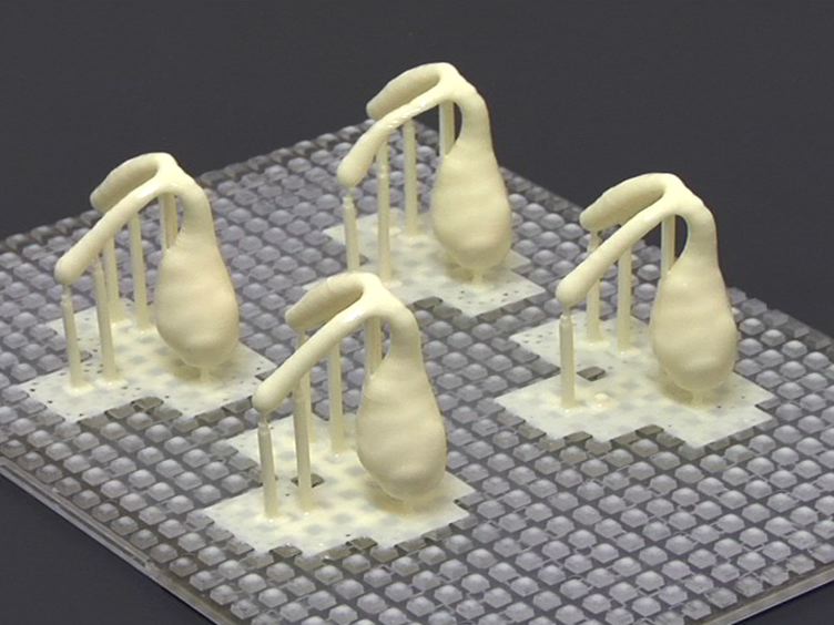
The top panel of Figure 7 illustrates visual renderings of two digital embryos, and the bottom panel of Figure 7 illustrates the corresponding printouts generated by a commercially available 3-D prototyper.
Figures 8 and 9 illustrate the procedures described in Section 6 for using image fragments to categorize a given visual object.

Figure 1. Virtual morphogenesis. The bottom panel illustrates a type of novel, naturalistic, virtual 3-D objects called "digital embryos"14. Digital embryos can be generated by simulating one or more of some of the key processes of biological embryogenesis: morphogen-mediated cell division, cell growth, cell movement and programmed cell death7,8,36,37. Each run starts with an icosahedron (shown in the top panel), and generates a unique embryo, depending on the VM parameter settings (or the 'genotype') of that embryo. Thus, the 16 embryos in the bottom panel have different shapes, because they all have different genotypes. Note that simpler or more complex shapes can be generated as needed (e.g., to optimally stimulate neurons at a given level of the visual hierarchy) by manipulating the genotype of the embryo. All of the aforementioned embryogenetic processes except programmed cell death were simulated in generating the embryos shown. Simulated programmed cell death is especially useful for creating targeted indentations (not shown).

Figure 2. Creating visual stimuli using digital embryos. Like any virtual 3-D object, digital embryos can be graphically manipulated to create visual scenes of arbitrary complexity using any standard 3-D graphical toolkit. This figure illustrates some common manipulations. (A) The same digital embryo is textured using many different textures, and lit from an invisible light source at top left. (B) A camouflaged scene is created by resizing and re-orienting the digital embryo and digitally placing it against the same background it was textured with. The digital embryo can be found in 'plain view' in the lower right quadrant. For additional examples of visual stimuli created using digital embryos, see refs. 9,10,12-14,38.

Figure 3. Creating digital embryo categories using VP. The VP algorithm emulates biological evolution, in that in both cases, novel objects and object categories emerge as heritable variations accumulate selectively. At each generation Gi , selected embryos procreate, leading to generation Gi+1. The progeny inherit the shape characteristics of their parent, but accrue shape variations of their own (as determined by small variations in their genotype) as they develop. This figure shows a 'family tree' of three generations of descendants starting from a single common ancestor, an icosahedron. Note that, in this case, the shape complexity increases from the icosahedron to generation G1, but not from G1 onward. This is because increase in cell numbers (i.e., cell division) was allowed from the icosahedron to generation G1, but not from G1 onward. In general, cell division tends to increase shape complexity, whereas other morphogenetic processes such as cell movement and cell growth change shape without changing the overall complexity of the shape.

Figure 4. VP using virtual objects other than digital embryos. This figure helps illustrate the general principle that virtual objects other than digital embryos can be used as input to VP. The VP algorithm in its current form can operate on any virtual 3-D object whose surface consists solely of triangles. Generation G1 comprised of (from left to right) a gourd, diamond, face mask, apple, rock, and cactus. Note that the objects in generation G1 in this figure do not have a common ancestor, because VP does not require it. Objects in G2 and G3 represent the descendants of the rock in G1. No cell divisions were allowed in any generation, so that all shape variations arose solely from the movement and/or growth of the individual 'cells' of the given object.

Figure 5. Using morphing to create smooth variations in shape. Morphing involves taking two given objects (far left and far right embryo in this figure) and calculating the intermediate objects (intervening embryos) by interpolating between the corresponding vertices of the two designated objects. In the case shown, all vertices were interpolated using the same scalar factor, resulting in a linear morphing. However, it is also possible to morph the objects non-linearly (not shown). Morphing is computationally straightforward when there is an exact one-to-one correspondence between the vertices of two objects, as in the case shown. However it is possible, in principle, to morph between any two given virtual objects regardless of whether their vertices correspond exactly, although there is no unique principled method for doing so17,18.

Figure 6. Using principal components to create smooth variations in shape. (A) Average embryo. This embryo represents the arithmetic average of 400 embryos (200 each from categories K and L in Figure 3). Principal components were calculated as described in Step 4.3. Note that principal components represent mutually independent, abstract shape dimensions of the 400 embryos (not shown)25,26. 400 embryos yield 399 non-zero principal components25,26, which together account for all the variance, or the shape information, available collectively in the embryos. By convention, principal components are arranged in the decreasing order of their eigenvalues, or the proportion of the overall variance they explain25,26. In this case, the first two principal components respectively accounted for 73% and 19% of the shape information available in the 400 embryos. (B) Embryos that represent different weights (or more precisely, weighted eigenvalues) of Principal Component 1. The weights varied from +2 (far left) to -2 (far right) in equal steps of -0.2. (C) Embryos that represent different weights of Principal Component 2. The weights also varied from +2 (far left) to -2 (far right) in equal steps of -0.2. Note that manipulating principal components does not exclusively manipulate any given specific body part of the embryo (e.g., the wings of the embryo in the case shown). However, if necessary, body parts of virtual 3-D objects can be manipulated in any arbitrary user-defined fashion using most of the commercially available 3-D modeling environments (not shown).

Figure 7. Creating haptic objects. Virtual 3-D objects can be 'printed' as haptic objects using a standard, commercially available 3-D 'printer' or prototyper. This figure shows digital embryos rendered as visual objects (top row) or as the corresponding haptic objects (bottom row). The haptic objects shown in this figure were printed to be about 6 cm wide (scale bar = 1 cm), although the objects can be printed at much smaller or larger sizes.

Figure 8. A template for an example informative fragment. In this example, the template has a threshold of 0.69 associated with it.

Figure 9. A new image for which the object category is not known and needs to be determined.
Discussion
Usefulness of VM and VP in Cognitive Science Research
We have previously described the usefulness of VM and VP in detaill9,10,12-14. Briefly, VM, especially the digital embryo methodology, is useful because it provides a principled and flexible method for creating novel, but naturalistic 3-D objects14. Similarly, VP provides a principled method of creating naturalistic categories9,10,12,13. It is worth noting that object categories generated by VP share many features with object categories in nature, including the fact that the categories tend to be hierarchical in nature, and the feature variations within and across categories arise independently of the experimenter and the algorithms for classifying them39.
Current Limitations and Future Directions
Three current limitations of our protocol and the directions for future work they suggest are particularly noteworthy: First, both VM and VP simulate biological processes. While we show that non-biological virtual objects can be used as substrates for these processes, the underlying processes are still biologically motivated. However, natural objects - biological and non-biological alike - undergo shape changes due to non-biological forces. For instance, rocks may change in shape due to geological processes such as erosion or sedimentation. New categories of rock may arise from other such geological processes. It should be relatively straightforward to incorporate these processes into the repertoire of available shape change algorithms.
The second major limitation of our protocol is that its current repertoire of dynamic shape changes is rather limited. It is desirable to incorporate a larger array of shape changes, such as biological motion, or motion due to external forces such as wind, water or gravity. We expect that it will be relatively straightforward to bring to bear the known computer animation algorithms to implement such dynamic shape changes.
The third major limitation of our protocol is that VM currently does not include many other known morphogenetic processes including, most notably, gastrulation36. It also fails to incorporate some known constraints, such as the fact that morphogenesis in plants is mediated entirely by growth, with little or no cell movement possible, because of the cell walls36. Similarly, VP does not include other known phylogenetic processes such as genetic drift40. Addressing these limitations would help greatly facilitate the use of our protocol in developmental, ecological and evolutionary simulations.
Disclosures
No conflicts of interest declared.
Acknowledgments
This work was supported in part by the U.S. Army Research Laboratory and the U. S. Army Research Office grant W911NF1110105 and NSF grant IOS-1147097to Jay Hegdé. Support was also provided by a pilot grant to Jay Hegdé from the Vision Discovery Institute of the Georgia Health Sciences University. Daniel Kersten was supported by grants ONR N00014-05-1-0124 and NIH R01 EY015261 and in part by WCU (World Class University) program funded by the Ministry of Education, Science and Technology through the National Research Foundation of Korea (R31-10008). Karin Hauffen was supported by the Undergraduate Research Apprenticeship Program (URAP) of the U.S. Army.
Materials
| Name | Company | Catalog Number | Comments |
| Digital Embryo Workshop (DEW) | Mark Brady and Dan Gu | This user-friendly, menu-driven tool can be downloaded free of charge as Download 1 from http://www.hegde.us/DigitalEmbryos. Currently available only for Windows. | |
| Digital embryo tools for Cygwin | Jay Hegdé and Karin Hauffen | This is a loose collection of not-so-user-friendly programs. They are designed to be run from the command-line interface of the Cygwin Linux emulator for Windows. These programs can be downloaded as Download 2 from http://www.hegde.us/DigitalEmbryos. The Cygwin interface itself can be downloaded free of charge from www.cygwin.com. | |
| Autodesk 3ds Max, Montreal, Quebec, Canada | Autodesk Media and Entertainment | 3DS Max | This is a 3-D modeling, animation and rendering toolkit with a flexible plugin architecture and a built-in scripting language. Available for most of the current operating systems. |
| MATLAB | Mathworks Inc., Natick, MA, USA | MATLAB | This is a numerical computing environment and programming language with many useful add-on features. Available for most of the current operating systems. |
| R statistical toolkit | R Project for Statistical Computing | R | Can be downloaded free of charge from http://www.r-project.org/. Available for most of the current operating systems. |
| OpenGL | Khronos Group | OpenGL | This cross-language, cross-platform graphical toolkit can be downloaded free of charge from www.opengl.org. |
| V-Flash Personal Printer | 3D Systems Inc., Rock Hill, SC, USA | V-Flash | This is a good value for all 3-D printing applications described in this report. The print materials are also vended by 3D Systems, Inc. Less expensive models are available in open source form from RepRap (rapmanusa.com) and MakerGear. More expensive models (> $30 K) are available from Objet Geometries, 3DS Systems, Z-Corp, Dimension Printing etc. |
| TurboSquid.com | TurboSquid Inc., New York, LA | (various objects) | Various virtual 3-D objects can be downloaded from this site free of charge or for a fee. |
| Table 1. Table Of Specific Toolkits And Equipment. | |||
References
- Palmeri, T. J., Gauthier, I. Visual object understanding. Nat. Rev. Neurosci. 5, 291-303 (2004).
- Seger, C. A., Miller, E. K. Category learning in the brain. Annu. Rev. Neurosci. 33, 203-219 (2010).
- Perceptual Learning. Fahle, M., Poggio, T. , MIT Press. (2002).
- Ashby, F. G., Maddox, W. T. Human category learning. Annu. Rev. Psychol. 56, 149-178 (2005).
- Gauthier, I., Tarr, M. J. Becoming a "Greeble" expert: exploring mechanisms for face recognition. Vision Res. 37, 1673-1682 (1997).
- Op de Beeck, H. P., Baker, C. I., DiCarlo, J. J., Kanwisher, N. G. Discrimination training alters object representations in human extrastriate cortex. J. Neurosci. 26, 13025-13036 (2006).
- Cui, M. L., Copsey, L., Green, A. A., Bangham, J. A., Coen, E. Quantitative control of organ shape by combinatorial gene activity. PLoS Biol. 8, e1000538 (2010).
- Green, A. A., Kennaway, J. R., Hanna, A. I., Bangham, J. A., Coen, E. Genetic control of organ shape and tissue polarity. PLoS Biol. 8, e1000537 (2010).
- Hegdé, J., Bart, E., Kersten, D. Fragment-based learning of visual object categories. Curr. Biol. 18, 597-601 (2008).
- Fragment-based learning of visual categories. Bart, E., Hegdé, J., Kersten, D. Cosyne 2008 Conference, 2008 Feb 28-Mar 2, Salt Lake City, , Cosyne. Salt Lake City. 121-12 (2008).
- Ball, P. Nature's patterns : a tapestry in three parts. , Oxford University Press. (2009).
- Vuong, Q. C. Visual categorization: when categories fall to pieces. Curr. Biol. 18, 427-429 (2008).
- Kromrey, S., Maestri, M., Hauffen, K., Bart, E., Hegde, J. Fragment-based learning of visual object categories in non-human primates. PLoS One. 5, e15444 (2010).
- Brady, M. J., Kersten, D. Bootstrapped learning of novel objects. J. Vis. 3, 413-422 (2003).
- Blanz, V., Vetter, T. A morphable model for the synthesis of 3D faces. SIGGAPH. 26, 187-194 (1999).
- Freedman, D. J., Riesenhuber, M., Poggio, T., Miller, E. K. Categorical representation of visual stimuli in the primate prefrontal cortex. Science. 291, 312-316 (2001).
- Lerios, A., Garfinkle, C. D., Levoy, M. Feature-based volume metamorphosis. SIGGRAPH. , 449-456 (1995).
- Bronstein, A. M., Bronstein, M. M., Kimmel, R. Numerical geometry of non-rigid shapes. , Springer. (2008).
- Lotka, A. J. Natural Selection as a Physical Principle. Proc. Natl. Acad. Sci. U.S.A. 8, 151-154 (1922).
- Duda, R. O., Hart, P. E., Stork, D. G. Pattern classification. , 2nd edn, Wiley. (2001).
- Bishop, C. M. Pattern recognition and machine learning. , Springer. (2006).
- Theodoridis, S., Koutroumbas, K. Pattern recognition. , 3rd edn, Academic Press. (2006).
- Sokal, R. R. Biometry : The principles and practice of statistics in biological research. , 4th edn, W.H. Freeman and Co. (2011).
- Tuffery, S. Data mining and statistics for decision making. , Wiley. (2011).
- Crawley, M. J. Statistical Computing: An Introduction to Data Analysis using S-Plus. , Wiley. (2002).
- Venables, W. N., Ripley, B. D. Modern Applied Statistics with S. , Springer. (2003).
- Beier, T., Neely, S. Feature-based image metamorphosis. SIGGRAPH. 26, 35-42 (1992).
- Kent, J. R., Carlson, W. E., Parent, R. E. Shape transformation for polyhedral objects. SIGGRAPH. 26, 47-54 (1992).
- Gomes, J. Warping and morphing of graphical objects. , Morgan Kaufmann Publishers. (1999).
- Ullman, S. Object recognition and segmentation by a fragment-based hierarchy. Trends Cogn. Sci. 11, 58-64 (2007).
- Kobatake, E., Tanaka, K. Neuronal selectivities to complex object features in the ventral visual pathway of the macaque cerebral cortex. J. Neurophysiol. 71, 856-867 (1994).
- Serre, T., Wolf, L., Poggio, T. Proceedings of 2005 IEEE Computer Society Conference on Computer Vision and Pattern Recognition (CVPR). , IEEE Computer Society Press. (2005).
- Ullman, S., Vidal-Naquet, M., Sali, E. Visual features of intermediate complexity and their use in classification. Nat. Neurosci. 5, 682-687 (2002).
- Davis, M. J. Computer graphics. , Nova Science Publishers. (2011).
- Lengyel, E. Mathematics for 3D game programming and computer graphics, third edition. , 3rd Ed, Cengage Learning. (2011).
- Gilbert, S. F. Developmental biology. , 9th edn, Sinauer Associates. (2010).
- Gilbert, S. F., Epel, D. Ecological developmental biology : integrating epigenetics, medicine, and evolution. , Sinauer Associates. (2009).
- Hegdé, J., Thompson, S. K., Brady, M. J., Kersten, D. Object Recognition in Clutter: Cortical Responses Depend on the Type of Learning. Frontiers in Human Neuroscience. 6, 170 (2012).
- Mervis, C. B., Rosch, E. Categorization of natural objects. Annual Review of Psychology. 32, 89-115 (1981).
- Futuyma, D. J. Evolution. , 2nd edn, Sinauer Associates. (2009).