1
Institut für Biologie – Neurobiologie, Freie Universität Berlin, Germany
2
Bernstein Center for Computational Neuroscience, Berlin, Germany
In their natural environment, many insects need to identify and evaluate behaviorally relevant odorants on a rich and dynamic olfactory background. Behavioral studies have demonstrated that bees recognize learned odors within <200 ms, indicating a rapid processing of olfactory input in the sensory pathway. We studied the role of the honeybee antennal lobe network in constructing a fast and reliable code of odor identity using in vivo intracellular recordings of individual projection neurons (PNs) and local interneurons (LNs). We found a complementary ensemble code where odor identity is encoded in the spatio-temporal pattern of response latencies as well as in the pattern of activated and inactivated PN firing. This coding scheme rapidly reaches a stable representation within 50–150 ms after stimulus onset. Testing an odor mixture versus its individual compounds revealed different representations in the two morphologically distinct types of lateral- and median PNs (l- and m-PNs). Individual m-PNs mixture responses were dominated by the most effective compound (elemental representation) whereas l-PNs showed suppressed responses to the mixture but not to its individual compounds (synthetic representation). The onset of inhibition in the membrane potential of l-PNs coincided with the responses of putative inhibitory interneurons that responded significantly faster than PNs. Taken together, our results suggest that processing within the LN network of the AL is an essential component of constructing the antennal lobe population code.
Honeybees (Apis mellifera) are social insects that use odors as communication signals. These odors are of simple structure, typically composed of a single chemical compound. On the contrary, naturally occurring odorants that become relevant for the bee during foraging are generally complex blends of a large number of volatile compounds (Pichersky and Gershenzon, 2002
) with time-varying composition and concentrations. Psychophysical studies in bees (Chandra and Smith, 1998
; Deisig et al., 2003
), catfish (Valenticic et al., 2000
), and humans (Livermore and Laing, 1998
) have shown that the neural representation of an odor mixture can be synthetic or elemental whereby the mixture either acquires a novel perceptual quality or it resembles its elemental compounds. In vertebrates, odor mixture interactions were observed at different levels of the olfactory system, in the periphery (Duchamp-Viret et al., 2003
), in the olfactory bulb (Davison and Katz, 2007
; Giraudet et al., 2002
; Lin et al., 2006
; Tabor et al., 2004
) and in the olfactory cortex (Lei et al., 2006
; Zou and Buck, 2006
). Studies of mixture interaction in the honeybee antennal lobe using Ca2+-imaging of glomerular activity revealed suppressive interactions in which the response to an odor mixture can be much lower than the response to the single compounds (Deisig et al., 2006
; Joerges et al., 1997
; Silbering and Galizia, 2007
). Such a suppression effect was not observed in the moth Spodoptera littoralis where glomerular Ca responses to mixtures always demonstrated hypoadditive interactions resembling the response to the strongest compounds within the mixture (Carlsson et al., 2007
).
Animals have evolved sophisticated mechanisms to distinguish naturally occurring odors, and to extract meaningful information from a rich olfactory environment. Recent behavioral studies could show that a perceptual discrimination of odors occurs rapidly after the onset of an odor stimulation. Mice are able to discriminate dissimilar odors within <250 ms (Abraham et al., 2004
) and they can distinguish a novel odor from learned odors within only 140 ms (Wesson et al., 2008
). A recent study in honeybees has demonstrated their ability to distinguish between different olfactory stimuli that are as short as 200 ms (Wright et al., 2009
). Consistent with this result, we found that mushroom body (MB) extrinsic neurons in the honeybee reliably signal the presence of a conditioned odor within <200 ms after stimulus onset (Pamir et al., 2008
; Strube-Bloss et al., 2008
). Thus, odor processing in the olfactory pathway must be fast and lead to a reliable code of odor identity at the input level to the central brain structures.
The olfactory system of the honeybee comprises 60,000 olfactory sensory neurons (OSNs; Esslen and Kaissling, 1976
), which are located predominantly in pore plate sensillae on the antennae. Each OSN conveys the olfactory information through one of the four antennal tracts (T1-4, Figure 1
A) and innervates neurons in one of ∼160 glomeruli (Arnold et al., 1985
; Flanagan and Mercer, 1989
; Kelber et al., 2006
). Glomeruli receiving input from T1 OSN are located in the ventral–rostral hemisphere of the AL whereas glomeruli which receive input from T2-4 glomeruli in the dorsal–caudal hemisphere (Figure 1
A; Kirschner et al., 2006
). Glomeruli represent synaptic interaction sites between the OSN, a total of ∼4000 AL-intrinsic local interneurons (LNs, Figure 1
B, depicted in red; Fonta et al., 1993
) and ∼950 projection neurons (PNs, Figures 1
C,D; Kirschner et al., 2006
; Rybak and Eichmueller, 1993
). Anatomically we distinguish two types of PNs. The lateral PNs (l-PNs) receive input exclusively from T1 glomeruli (Figure 1
A, green circle) and send their axons along the lateral antennocerebralis tract to the higher order brain centers, the lateral horn (LH) and the MB. The median PNs (m-PNs) exclusively originate in T2-4 glomeruli (Figure 1
A, purple circle) and project along the median antennocerebralis tract, first to the MB and then to the LH (Abel et al., 2001
; Bicker et al., 1993
; Kirschner et al., 2006
; Mobbs, 1982
; Müller et al., 2002
). Each uniglomerular PN is therefore identified by the respective glomerulus and numbered according to the 3-D Atlas of the honeybee AL (Figures 1
C,D; Galizia et al., 1999
).
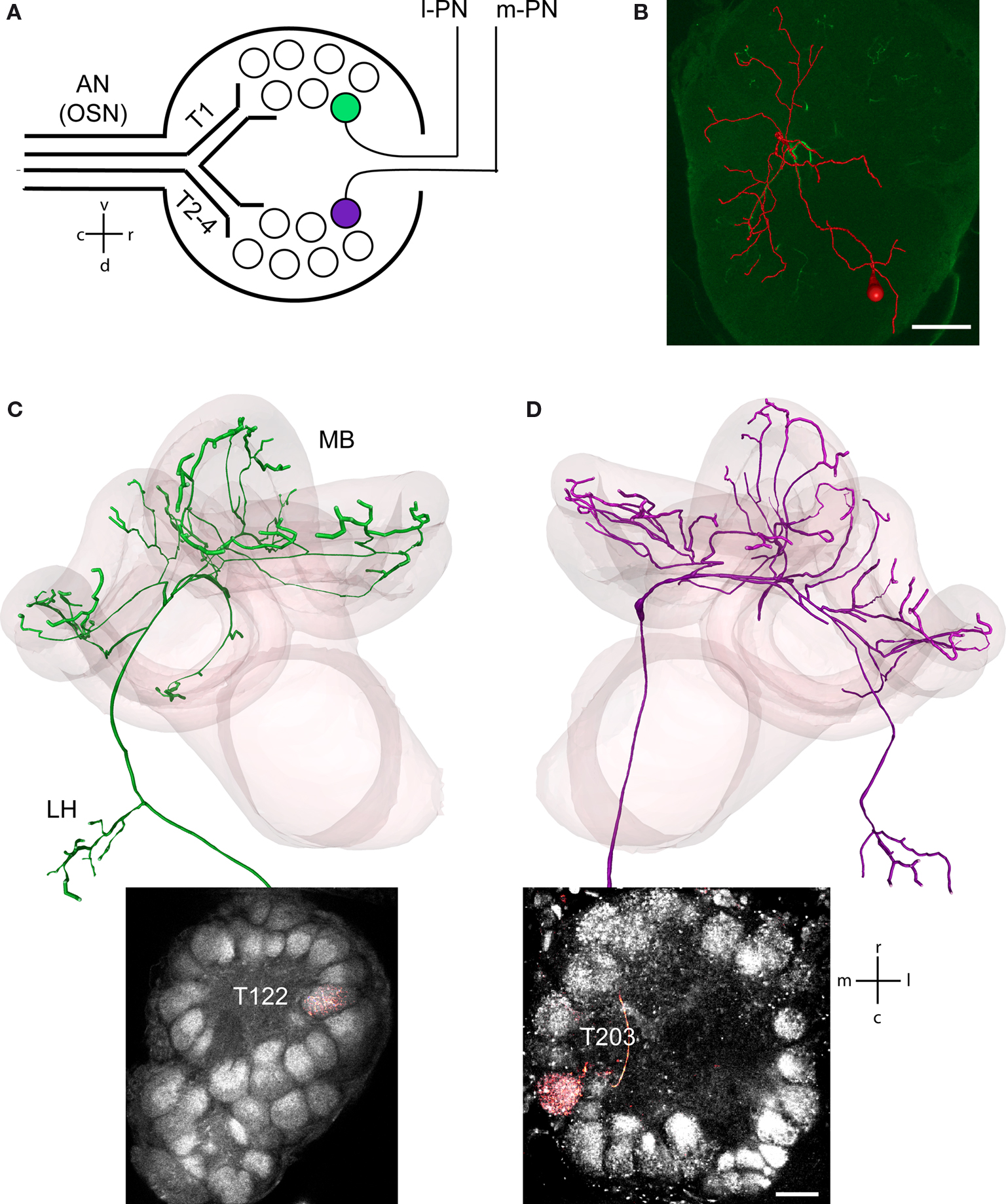
Figure 1. Identification of l-PNs, m-PNs and LNs within the glomerular organization of the AL. (A) Schematic drawing of the glomerular organization within the AL. OSN enter the AL via four antennal nerve (AN) tracts (T1-4) and terminate within glomeruli of two separate AL hemispheres. l-PNs have their uniglomerular arborizations within T1 glomeruli (green) whereas m-PNs within T2-4 glomeruli (purple). (B) 3-D reconstruction of an intracellular filled LN.
(C) l-PN identified by its uniglomerular projections within the T1-22 glomerulus stained with Micro-Ruby. The 3-D reconstruction shows that l-PNs leave the AL via the lateral antennocerebralis tract projecting first to the lateral horn (LH) and then to the mushroom bodies (MBs). (D) m-PN identified by its uniglomerular projections within the T2-03 glomerulus stained with Micro-Ruby. 3-D reconstruction shows that m-PNs leave the AL via the median antennocerebralis tract projecting first to the MBs and then to the LH. Scale bar B = 100 μm, D = 30 μm.
In the present study, we performed intracellular recordings of single l-PNs, m-PNs and LNs and analyzed their spatio-temporal responses to odors and odor mixtures. We specifically addressed the following questions. How fast does an ensemble code evolve in a population of PNs? Is there a functional distinction between the two anatomically distinct types of PNs? With regard to mixture encoding we confirmed the hypothesis that l-PNs can show mixture suppression as previously reported in Ca-imaging studies at the glomerular level, and we tested whether this effect does carry over to the m-PNs. Finally, we asked whether local inhibition with in the AL network underlies response suppression in individual PNs.
Honeybees
Worker bees (A. mellifera carnica) were caught at the hive entrance or in an indoor flight room, immobilized by cooling, and mounted in plastic tubes. The bees were fed with sucrose solution and kept in the dark at 20°C and high humidity. On the following day, the head was fixed with wax and opened between the median ocellus and the base of the antennae. Glands and tracheal sheaths were removed. A second hole was cut to expose the esophagus and to stretch it aiming to reduce movement of the brain. The brain was kept wet at all times by dribbling drops of bee physiological saline solution onto (in mmol–1: 130 NaCl, 6 KCl, 2 MgCl2, 10 HEPES, 17 glucose, 6 fructose, 160 sucrose, pH 6.7).
Electrophysiology
Glass electrodes were pulled with a horizontal laser puller (P-2000 Sutter Instruments, Novato, CA, USA) and their tips were filled with 4% tetramethylrhodamine-biotin dextran (Micro-Ruby; Invitrogen, Germany) in 0.2 M potassium acetate. The electrodes (resistance 120–200 MΩ) were positioned at the top of the AL by using a micromanipulator (Leitz) and lowered posteriorly into the neuropil until a neuron could be penetrated. A reference electrode, a chlorized silver wire, was inserted into the eye. The recordings were done in bridge mode using an intracellular BRAMP 1 amplifier (NPI Electronics, Tamm, Germany). Data were, digitized using a 1401 interface and stored on a PC using spike2.5 software (Cambridge Electronic Design, UK).
Neuron Identification
Single l- and m-PNs were intracellular stained by injecting Micro-Ruby iontophoretically using depolarizing current pulses with a duration of 0.2 s applied at 1–2 Hz. Successful staining allowed the identification of the PN type (l or m) by location of their uniglomerular projections (Figures 1
C,D) (l-PNs receive input from T1 glomeruli whereas m-PNs from T2-T4 glomeruli, see Figure 1
A). Intracellular recording and filling (approximate recording time >10 min, approximate staining time ∼20 min) was performed intra-axonally. Due to the small axon diameter (∼3–5 μm), recording conditions were extremely difficult, strongly limiting the overall experiment time. We kept stimulus protocols short to ensure sufficient time for the iontophoresis. In cases of highly stable recording conditions, we increased the stimulus protocol to either comprise a larger stimulus set or to increase number of repetitions for a subset of the stimuli. Successful staining could be achieved in about 50% of all neurons. Since the antennal lobe of the honeybee is well described (Abel et al., 2001
; Galizia et al., 1999
; Kirschner et al., 2006
) identification of l- and m-PNs was alternatively performed by the spatial position of the electrode with respect to the hemispherical segregation of T1 and T2-4 glomeruli (T1 = ventral–rostral, T2-4 = dorsal–caudal). LNs could easily be identified either by their specific intracellular action potential waveform and their firing pattern which clearly differ from those of the PNs (Galizia and Kimmerle, 2004
). Previous imaging studies of the AL could only resolve signals from the T1 glomeruli but not form T2-4. We therefore preferentially targeted m-PNs that innervate T2-4. In total we identified and analyzed PNs: N = 7 (l-type), N = 23 (m-type); and LNs: N = 7.
Odor Stimulation
The animal’s antennae were exposed to a constant active charcoal-filtered stream of room air (airflow rate 10 ml/s) guided through a glass tube with an inner diameter of 14 cm placed 1 cm from the antenna. For each odor, 4 μl were placed on a filter paper in a glass syringe, which was introduced into the continuous air stream. The control stimulus was a glass syringe plus filter paper with mineral oil (Sigma-Aldrich, Germany) delivering a constant airflow rate of 10 ml/s. To avoid mechanical stimulation a computer-controlled valve switched between control stimulus and odor-loaden syringe such that the antenna was always exposed to an air stream with a flow rate of 20 ml/s. The stimulus timing was computer-controlled and each odor stimulation lasted for 2 s. The delay from the onset trigger for valve opening to the arrival of the odorant at the antenna was estimated as ∼200–220 ms. For response latency analyses and display purposes we therefore subtracted a fix delay of 200 ms from the measured latencies. All odors were diluted 1:10 in mineral oil and checked for purity and mixture composition by gas chromatography (Trace GC Ultra, Thermo, Electron Corporation, Waltham, MA, USA). The animals’ antennae were stimulated with a tertiary mixture and its elemental compounds as well as other single compound odors and complex odor mixtures (Sigma-Aldrich, Germany). The tertiary mixture was composed of the blossom compounds nonanol and hexanol and 2-heptanon, which is known to be a compound of the alarm pheromone in bees (Balderrama et al., 2002
). Additionally natural floral blends as well as single compounds exhibiting different functional groups were tested. In some animals multiple-trial presentations of the same odor were used to test response reliability, whereas in other animals one-trial presentation (in some cases with few repetitions) of different odors (between 2 and 30) were performed in a randomized fashion. We analyzed only stable recordings that lasted for at least 10 min.
Data Analysis
Matlab and the Matlab Statistics Toolbox (The MathWorks, Inc.) were used for the analysis of the intracellular voltage traces and spike trains. We implemented all custom-written algorithms used for analysis in the present manuscript in the FIND open source Matlab toolbox for neural data analysis (Meier et al., 2008
; http://find.bccn.uni-freiburg.de/
).
Firing rate analysis
Intracellular spikes times were detected with a threshold criterion. Firing rates were measured by convoluting single trial spike trains with a kernel of asymmetric shape k(t) = t × exp(−t/τ) and time resolution τ, defined on a finite support (Nawrot et al., 1999
; Parzen, 1962
). We aligned the resulting rate function at time w that indicates the center of mass of the kernel (w = 42 ms for τ = 25 ms). For color-coded representation of excitatory and inhibitory responses, we subtracted from the response the baseline rate measured during 1 s preceding the stimulus. We then represent the rate response of a neuronal ensemble with n neurons to odor stimulus a at any given point in time as the n-dimensional rate vector va. We then define the distance between two rate vectors va, vb as dab = Σ |via − vib|.
Response latency analysis
To estimate absolute and relative trial-by-trial latencies we used a method that we described in detail elsewhere (Meier et al., 2008
). A demo script for this method together with a demo data set is available online at the official website of the FIND toolbox (http://find.bccn.uni-freiburg.de/?n=Docu.Tutorial
). In a first step, we estimated from a given single trial spike train the time derivative of the signal by convolution with an asymmetric Savitzky–Golay filter (Savitzky and Golay, 1964
) (polynomial order 2, width 300 ms, Welch windowed). In a second step, we estimated the N-1 relative latencies of the individual spike trains. For this we used an algorithm that allows to optimally align all N single trial derivatives (taking into account the first 700 ms) such that their pair-wise cross-correlation is maximized (Nawrot et al., 2003
). The resulting optimal N-1 time-shifts correspond to the relative latencies and we measured their standard deviation σ to quantify the cross-trial latency variability. In a third step, we aligned in time all individual single trials according to the optimal time shifts (with a zero mean shift to preserve the center of mass) and then merged all single trial spike trains into 1.
For each odor, we thus obtained one trial-aligned and merged spike train. To obtain the relative latencies across different odors we repeated the same procedure but now using the merged spike trains. We again used the standard deviation to quantify latency variability across odors. To test for the significant difference of two distributions of latency differences we used the Kolmogorov–Smirnov test. To obtain the absolute response latency for each neuron as averaged across all odors we optimally aligned the odor-specific spike trains as described above and merged all spike trains. We then computed the time derivative of the firing activity as explained above and measured the peak time of the maximum. We defined this point in time at which the rise of the response was steepest as the absolute single neuron latency. Absolute latency estimates have a small but fix bias toward slightly higher values as we subtracted the lower limit of the estimated delay for odor delivery (200 ms), and because of the asymmetry of the Savitzky–Golay filter kernel.
Before estimating the latency of intracellular inhibition the membrane potential of PNs was low-pass filtered with a cut-off frequency of 100 Hz using an exponential impulse response kernel (decay time constant 1.6 ms). Response onset was then determined as the time of crossing a threshold defined as the average baseline response (during 5 s preceding stimulus onset) minus either one or two times the standard deviation during baseline period (excluding APs).
Specificity index
We defined the specificity index s of a neuron as the number of odors that evoked either an excitatory (sex) or inhibitory (sin) response (within the first second after stimulus onset) divided by the total number of tested odors. For each type of PNs we computed the specificity index separately for single compound and odor mixture presentations.
Mixture index
To quantify the response difference between mixture and most effective compound we calculated the mixture index κ = (y − x)/(x + y) where x denotes the absolute number of response spikes for the individual odor compound that yielded the strongest response and y denotes the absolute number of spikes in the response to the mixture, counted in a fix interval from 200 to 700 ms after stimulus onset at t = 0. κ Will be close to 0 in the case of a hypoadditive mixture response, and κ assumes values close to −1 (+1) in the case of a suppressive (additive) mixture effect. The distribution of κ values may be strongly skewed, in particular for values close to −1/1. Therefore, before averaging values of κ we applied Fisher’s z-transform. We tested for a deviation from the null hypothesis of two samples of κ having the same median using the Wilcoxon rank sum test.
l- and m-PN Odor Response Profiles
We performed intracellular recordings of single PNs and tested their dynamic responses elicited by single compound odors. l- and m-PNs were identified either by their uniglomerular arborizations, (Figures 1
C,D) or by the location of the particular recording site (see Section “Materials and Methods”). First, we characterized the response kinetics and response reliability of PNs. Both types of PNs typically exhibited a phasic–tonic spike response pattern that outlasted the stimulus presentation. Figures 2
A–D shows the response characteristics for a l-PN receiving input from the T1-22 glomerulus (Figures 2
A,B) and a m-PN receiving input from the T3-45 glomerulus (Figures 2
C,D). The responses were highly reliable across trials in all neurons tested. If a response was observed during one stimulus presentation, then it could reliably be detected in all of the trials. This is demonstrated in the spike raster diagrams of Figures 2
B,D. Based on this result we reduced the odor stimulus protocol to single or few trials of one and the same odor to test a larger set of odors within the limited experimental time. On average, the dynamic response profile of l- and m-PNs was very similar (Figure 2
E). The spontaneous firing rate was typically low with a mean of 6.8 spikes/s (median 3.4/s) and the average maximum responses peaked around 70 spikes/s. Several neurons showed no spontaneous spiking activity. Average response latencies of individual neurons were not significantly different (P = 0.7, Wilcoxon rank sum test) in l-PNs (148.3 ± 33 ms) and m-PNs (123.5 ± 14.6 ms) (Figure 2
F).
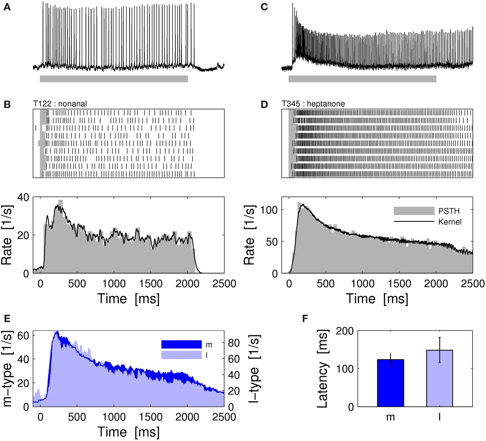
Figure 2. Odor response dynamics of projection neurons. (A) Intracellular membrane potential of one l-PN in response to the first presentation of the odor nonanal for 2 s (gray bar). Intracellular staining revealed that this neuron innervated the glomerulus T1-22. (B) The neuron responded reliably in all repeated presentations of the same stimulus (top). The individual single-trial latencies of response onset were estimated as indicated by the horizontal gray bars. The trial-averaged rate profile (bottom) shows a phasic–tonic response dynamics. (C) Intracellular response to 2-heptanon during the first trial and (D) repeated reliable responses of an identified m-PN that innervated the glomerulus T3-45. The rate profile indicates the initial phasic response followed by a tonic response that lasted throughout the static stimulus. (E) The average response rate profiles are of similar shape for l- (N = 7) and m-PNs (N = 23). (F) The response latencies of l-PNs are not significantly different from those of m-PNs (P = 0.7; Wilcoxon rank sum test). Average response latencies: 148.3 ± 33 ms (l-PN) and 123.5 ± 14.6 ms (m-PN). PSTH bin width: 20 ms; kernel resolution: τ = 14 ms.
Odor-Specific Response Latencies of l- and m-PNs
From behavioral experiments, it becomes evident that a code of odor identity must be rapidly established at the level of the AL output (see Section “Introduction”). We here consider one possible fast coding strategy, namely the encoding of odor identity in an odor-specific pattern of response latencies across an activated PN ensemble. To this end, we compared the differences in response latency as measured across different odors with the differences in latency across trials of repeated stimulus presentation. The experimental limitations of recording time made it necessary that we typically tested a diverse set of odors with very few trials or only very few odors during many trials. For a statistical evaluation, we therefore pooled all relative across-trial latencies (see Section “Materials and Methods”) separately for l- and m-PNs (Figures 3
A,B). The trial-to-trial variability of response onset was quantified by its standard deviation σ which was similar for both, l-PNs (Figure 3
A) and m-PNs (Figure 3
B) with σltrial = 22.5 ms and σmtrial = 28.3 ms, respectively. Next, we quantified the relative latencies across odors for each neuron and then pooled these again separately for the two types of PNs. The standard deviation of latencies across odors was considerably larger with σlodor = 41.6 ms (Figure 3
A) and σmodor = 49.2 ms (Figure 3
B). These latency differences across odors are significantly larger than across trials in both, l- and m-PNs (see Section “Materials and Methods”). Thus, on a statistical basis, response onset is odor-specific in both types of PNs. For the population of PNs this result immediately implies that there exists an odor-specific spatial latency pattern in the activated ensemble of uniglomerular PNs (cf. Figure 4
A) establishing a fast code of odor identity.
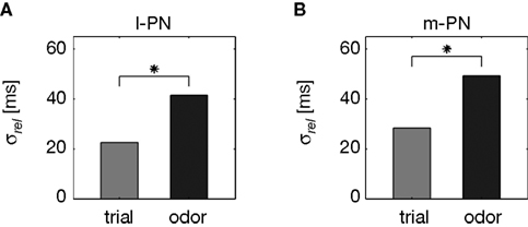
Figure 3. Odor-specific response latencies in projection neurons. Standard deviation σ of across-trial latencies (gray) and across-odor latencies (black) in l-PNs (A) (N = 62/29) and m-PNs (B) (N = 96/67). The differences of latencies across odors are significantly larger than the differences across trials (P < 0.01; Kolmogorov–Smirnov) for both types of PNs as indicated by the star in (A,B). The differences in latencies across trials were not significantly different for the two types of PNs (P > 0.05). See Section “Materials and Methods” for details on latency estimation.
l- and m-PN Responses in Space and Time
Results from Ca2+ imaging studies in the honeybee AL have shown odor-specific activation pattern of T1-glomeruli which are innervated by l-PNs. This suggests that odor identity is encoded by the activation of an odor-specific ensemble of PNs (Galizia and Menzel, 2000
; Joerges et al., 1997
; Sachse et al., 1999
). To test this hypothesis on the level of individual l- and m-PNs we performed two analyses. First, we concentrated on individual PNs and quantified their odor selectivity on the basis of mean responses during the first 800 ms after stimulus onset. For l- and m-PNs separately, we classified each response as inhibitory, excitatory or no response and defined the specificity index s, which represents the relative number of odors that elicited an excitatory (sex) or inhibitory response (sin) (see Section “Materials and Methods”). Our results show that on average l-PNs show an excitatory response to about half of the odors tested while m-PNs are less odor-specific with excitatory responses to about 2/3rd of the tested odors (cf. Table 1
; for examples see Figure 1
in Supplementary Material). Inhibitory responses (i.e., a suppressed spike rate) were observed in l-PNs for either 12% or 13% of the odors but they were very rarely observed in m-PNs and only for single compound odors but never in the case of an odor mixture. The odor-specific mean response classification of individual neurons necessarily translates into an odor-specific binary response pattern across the PN population.
Next, we examined the spatio-temporal activation in a pseudo population of non-simultaneously recorded l- and m-PNs and their responses to three single compound odors, the ketone 2-heptanon (2,7on) and the alcohols hexanol (6ol) and nonanol (9ol) (Figure 4
A). The color-coded response rate profiles in Figure 4
A indeed indicate that there exists a unique spatio-temporal pattern associated with each odor. A mean response classification (excitatory, inhibitory, no response) resulted in an odor-specific fingerprint (matrix in Figure 4
A). Since responses were highly reliable across repeated stimulations, this odor-specific spatial activation pattern will be identical in each trial. To investigate how the separations of odor-specific ensemble firing patterns evolve over time we computed the vector distance d in time-resolved fashion. In each point in time dab measures the distance between the vector of neuronal firing rates for two odors a and b. In each panel of Figure 4
B we show the average distance d′ = (dab + dac)/2 between the respective odor a and the two other compounds. The units of d represent the difference in firing rate per neuron, i.e., the number of spikes per second per neuron (see Section “Materials and Methods”). The resulting profiles in Figure 4
B display a highly dynamic behavior. The vector distance increases rapidly after stimulus onset and peaks at about 150∼250 ms. The highest divergence of odor response patterns naturally occurs only during the initial phasic responses. After about 300–500 ms the patterns again converge to reach an almost constant distance of ∼20 spikes/s associated with the tonic response that outlasted the stimulus.
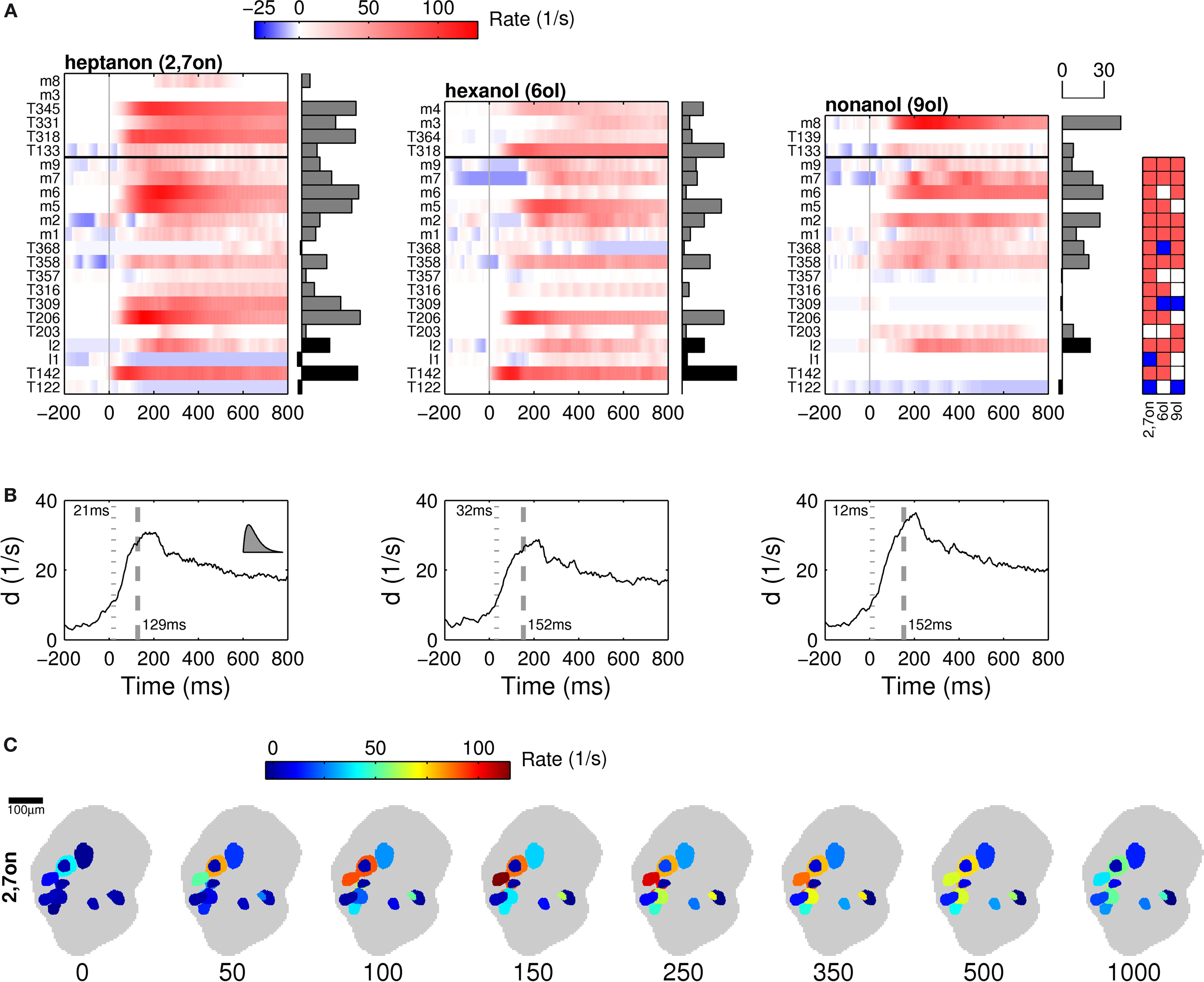
Figure 4. Population rate code in projection neuron ensembles. (A) Rate responses of PN populations to three different odors. Color code indicates rate deviation from the baseline as measured during the 500 ms preceding stimulus onset. Each row represents the firing rate of one individual neuron. The identification of each neuron is indicated on the left of each panel.
A subpopulation of N = 17 neurons (from bottom to horizontal black line) was tested with all three odors. The horizontal bars to the right of each panel indicate the response spike count within the first 500 ms after stimulus onset. The matrix on the right classifies for each neuron (vertical axis) and for each odor (horizontal) the type of rate response: excitatory (red), inhibited (blue) or neutral (white). The vertical columns thus represent a spatial fingerprint for the respective odor. (B) The time resolved distance d′ of the population rate vectors indicates the difference in firing rate per neuron (see text). In each panel, the dotted gray line and associated time stamp indicate the crossing of a threshold defined as mean plus five times the standard deviation as measured before stimulus onset. The dashed gray line indicates the time at which 90% of the maximum value was reached. Inset in left panel shows asymmetric shape of kernel function for rate estimation (τ = 25 ms) with correct temporal scale. (C) We translated the ensemble firing rates into a spatio-temporal rate code in the antennal lobe space by assigning to each neuron the corresponding 2-D section of the identified glomerulus (see Section “Materials and Methods”). The gray patch indicates a plane through the antennal lobe in the standard atlas of the honeybee brain. After each step of time from left to right we updated the color code according to the firing rate at the time indicated. A spatial map of the identified glomeruli (see Figure 2
in Supplementary Material) and additional video clips are available online in the “Supplementary Material.”
The spatial identification of l- and m-PNs by their uniglomerular arborizations further allowed us to establish a schematic map of the glomerular activation patterns within the AL. In Figure 4
C the spatio-temporal firing rate of identified PNs during the stimulation with 2-heptanon (2,7on) is shown as a glomerular activation pattern in eight successive time windows. Each time window represents in a color code the odor response for each individual PN at the location of the corresponding innervated glomerulus, resulting in a spatio-temporal activation pattern across all identified glomeruli. This interpretation assumes that the average PN activity of several uniglomerular neurons is highly similar to the response profile of the individual recorded neuron. Conversely, such a mapping can make a direct prediction for the glomerular response pattern in Ca-imaging studies that measure the mean activity of identified glomeruli.
Differential Odor Mixture Interactions in l- and m-PNs
Imaging studies in the honeybee AL revealed that T1-glomeruli often exhibit suppressed responses to a mixture but not to the elemental mixture components when presented alone (see Section “Introduction”). To test the prediction that this suppression effect is also evident at the level of single l-PNs, and to test whether it is also observable in individual m-PNs, which are not accessible by Ca-imaging in the AL, we compared individual l- and m-PN responses to an odor mixture and to its three elemental components when presented alone. Figures 5
A,B show the dynamic odor response profiles of one l- and one m-PN elicited by the tertiary mixture (black) and its compounds, the ketone 2-heptanon (green), and the alcohols hexanol (orange) and nonanol (blue). The l-PN showed excitatory responses to all three elemental compounds but was suppressed by their tertiary mixture (Figure 5
A). Note that the suppression is rapid such that not a single response action potential is elicited. The m-PN, however, showed excitatory responses to the odors hexanol, 2-heptanon and to the mixture, where the response to the mixtures resembled the stronger response to 2-heptanon (Figure 5
B).
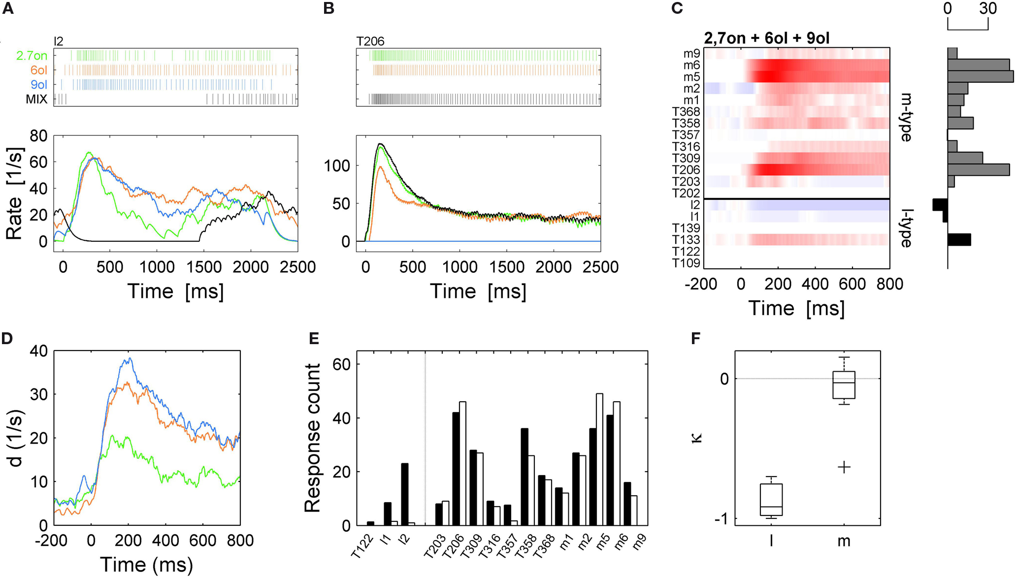
Figure 5. Different mixture effects in l- and m-PNs. (A) Single trial spike trains (top) and rate responses (bottom) of an l-PN to three odor compounds (heptanon = green, hexanol = orange, nonanol = blue) are excitatory while the response to the mixture (black) of all three odors is inhibited. (B) An example of an m-PN that shows an excitatory response to the same mixture (black) which closely resembles the most salient response to the elemental mixture compound heptanon. (C) Color-coded rate responses of 6 l-PNs and 13 m-PNs (separated by the blue horizontal line) in response to the same tertiary mixture. The l-PNs show mostly no or inhibited responses while the m-PNs show clear excitatory responses as indicated by the horizontal count bars. (D) Dynamics of the distance d between the ensemble response to the mixture and the ensemble response to each of the mixture elements for 15 neurons that were tested for all four odors. (E) Comparison of the absolute count measured during an initial response interval of 500 ms in response to the strongest compound (black) and the response count for the mixture (white) for all neurons that were tested in all conditions. The l-PNs indicate inhibited responses to the mixture, while the m-PNs indicate strong excitatory responses to the mixture. (F) The index κ measures the relative difference of mixture response and most salient response to an individual compound for all l- and m-PNs that were tested in all conditions.
The color-coded response profiles in Figure 5
C show the odor mixture responses across all PNs tested. The l-PNs were mostly inhibited or showed no response. In comparison, the majority of m-PNs showed a pronounced excitatory response. In Figure 5
D, we show the time resolved vector distance d. In each point in time, it measures the difference of the neuronal ensemble response to the mixture and its response to each of the individual compounds (cf. Figure 4
) as indicated by line color. The spatial response pattern for the mixture rapidly and strongly diverged from the response patterns of hexanol (orange) and nonanol (blue), and to a lesser degree from the response pattern of 2-heptanon (green).
We classified odor mixture responses according to three categories of mixture interactions: higher (synergy), equal (hypoadditivity) or lower (suppression) than the response to the most effective compound, following the conventions in (Duchamp-Viret et al., 2003
). For each l- and m-PN we determined the most effective compound, i.e., with the strongest response, and compared it with the response to the odor mixture. The bar diagram in Figure 5
E shows the response magnitude elicited by the odor mixture (white bars) and its strongest compound (black bars) indicating clear suppressive odor mixture interactions for all three l-PNs that we had tested for all compounds. In contrast, hypoadditive odor mixture interaction was observed in all m-PNs. For a quantitative analysis we determined the mixture interaction index κ as the relative difference of response magnitude between the mixture and the strongest compound (see Section “Materials and Methods”). The κ index reveals either synergistic (1), hypoadditive (0) or suppressive (−1) odor mixture interaction in each l- and m-PN tested. The l-PNs showed a clear suppressive interaction (κ = −0.98) in line with the prediction from imaging studies. Surprisingly, the m-PNs exhibited a clear hypoadditive interaction with average κ = −0.09 (Figure 5
F). This difference between l- and m-PN mixture interactions was significant (P < 0.01, Wilcoxon rank sum test). Synergistic odor mixture interactions were found in neither of the tested PNs. In Table 1
we listed the specificity index separately for single chemical compounds and mixtures that combined at least three such elementary compounds. It shows that only l-PNs exhibited inhibited responses to mixtures in 12% of all cases. Thus, our results for the l-PNs meet the prediction of previous imaging studies. The fact that we did not observe any suppressed response in all our m-PN recordings is a surprising and unexpected result, marking a functional difference of the two types of PNs.
Fast Inhibition in l-PNs Coincides with LN Responses
What could be the cause for the observed response suppression in l-PNs following odor mixture stimulation? Does suppression become effective at the level of OSNs or could local inhibition within the AL network explain the effect? To answer this question we first tested the intracellular membrane potential of PNs for signs of inhibition. The experimental setting for intracellular recordings from PNs makes it necessary to record from their individual axons. Thus, we recorded the membrane potential distal from the integrating segments and individual synaptic inputs could not be resolved. APs, however, were always detectable and in some cases we could observe clear hyperpolarizing deviations of the membrane potential that can be attributed to inhibitory inputs. In Figure 6
A we show six example traces from l-PNs with marked inhibition following stimulus onset. We can now see that the l-PN that innervates the T1-22 glomerulus is actually inhibited in response to the previously examined tertiary mixture. This was not visible in the rate response in Figure 5
C because of the low spontaneous activity level. We estimated the onset of the inhibitory compound by thresholding the membrane potential with respect to the mean and standard deviation prior to stimulus onset (see Section “Materials and Methods”). Surprisingly, we found that the response latency of the observed inhibition is on the order of only ∼60–90 ms and thus considerably shorter than the observed excitatory spike responses in PNs (Figure 2
). This explains why during mixture response suppression we did not observe a single response spike even in the initial response phase.
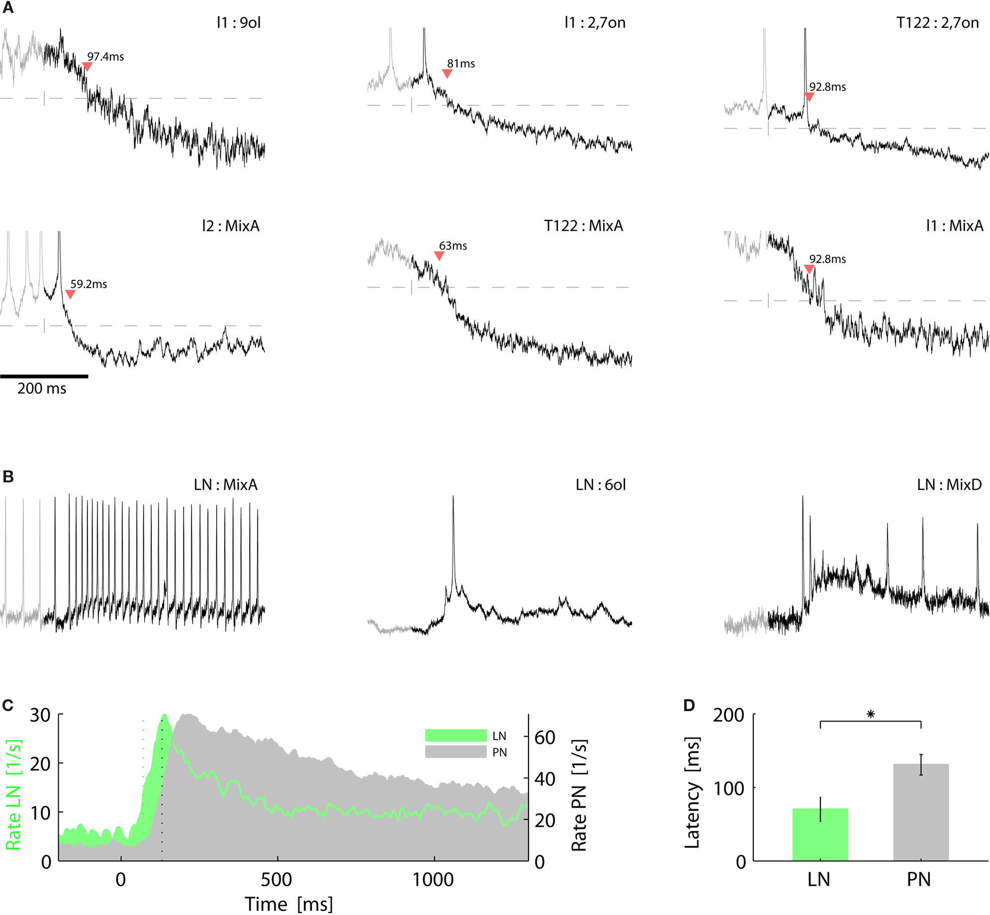
Figure 6. Fast inhibition can suppress projection neuron responses. (A) Membrane potential of individual l-type projection neurons during single trial responses to elemental odors (upper row) and to the same tertiary mixture as in Figure 5
(lower row). Stimulus onset (vertical dash) is followed by an inhibitory component that is detected by the crossing of the threshold (horizontal line, see Section “Materials and Methods”) as indicated by the red triangles and response latencies in ms. (B) Intracellular traces of three local interneurons show fast excitatory responses to single trial odor stimulation. Horizontal scale bar as in (A). (C) Average temporal firing rate profile of local interneurons (green) and projection neurons (gray) show that LNs respond faster than PNs and with a shorter phasic response. (D) Odor response latencies of LNs (70.0 ± 16.5 ms SEM; N = 6) are significantly (P < 0.05, Wilcoxon rank sum test) shorter than response latencies of PNs (130.8 ± 13.9 ms SEM; N = 30).
Could this fast inhibition of PNs be mediated by LNs? To answer this question we analyzed the onset latencies of excitatory spike responses in LNs. Figure 6
C shows the average dynamic rate profile of LNs (green) and PNs (gray). Indeed, the average latencies (vertical dotted lines) of LNs are significantly shorter than those of PNs with an average delay of Δt≈60 ms (Figure 6
D). The fast excitatory response of LNs to odor onset is also evident in the individual single trial traces shown in Figure 6
B. We may conclude that inhibitory interneurons in the AL can exhibit fast odor responses and are thus capable of rapidly and effectively suppressing PN responses.
We investigated the nature and dynamics of the encoding of single compound odors and odor mixtures in two morphological distinct types of PNs of the honeybee using in vivo intracellular recordings. Our results show that each odor activated a subset of PNs with each PN responding rather non-specifically to a number of odors. The spatial representation of odor identity in the PN ensemble evolves rapidly and peaks at about 150 ms after stimulus onset. PN activation involves a distinct odor-specific response latency, which implies an odor-specific pattern of relative latencies across the activated PN ensemble that is conveyed to higher order olfactory neuropils, the MB and the LH. Odor mixture representation depends on the type of PN, signifying a functional specialization of the two anatomically distinct neuron types. Our results indicate that l-PNs encode odor mixtures synthetically through a suppressed response to the mixture – an observation that was previously made on the level of average glomerular activity using Ca-imaging techniques – whereas m-PNs were never suppressed but encoded odor mixtures elementally, representing the strongest compound within the mixture (hypoadditive mixture interaction). Moreover, our results showed that synthetic odor mixture representation is associated with a prolonged hyperpolarization of the membrane potential, the onset of which in turn matched the stimulus-response latencies of LNs, which are significantly and considerably shorter than the ones observed in PNs. Therefore, we postulate that suppressive odor mixture interactions as observed in l-PNs arise from fast lateral inhibition mediated by the LN network.
Comparison with Imaging Studies
Part our results show that excitatory single neuron responses to individual odors organize into spatial patterns that involve about half of the PN population. Mixture suppression and inhibitory responses to complex odorants were confined to l-PNs. This part of our results is consistent with earlier imaging studies that could demonstrate the spatial representation of odors across T1 (l-PN) glomeruli in the honeybee AL (Deisig et al., 2006
; Galizia et al., 1999
; Joerges et al., 1997
; Sachse et al., 1999
) and suppressive odor mixture interaction in T1 glomeruli (Deisig et al., 2006
; Guerrieri et al., 2005
; Joerges et al., 1997
). However, the Ca-imaging methods used to monitor AL activity imposed several technical limitations. First, Ca-imaging yields only a limited temporal resolution that makes it difficult to assess the detailed dynamics with which a reliable representation emerges in the glomerular space. Second, during bath application of the Ca dye one generally cannot distinguish the types of neurons that were stained, PNs, LNs (excitatory or inhibitory), or glia (Heil et al., 2007
). Retrograde staining methods are likely to stain several PNs per glomerulus and thus average responses rather than single neuron responses are observed. Also, deliberate staining of LNs alone is difficult and thus no distinct conclusions on the dynamic involvement of LNs in the AL computations could be drawn. Finally, the imaging techniques used to measure glomerular activity could only resolve signals from the superficially located T1 glomeruli but not from T2-4 glomeruli. Thus, the odor response activity of local populations of m-PNs could not be tested in any of the mentioned studies. To overcome these limitations we carried out intracellular recordings. This allowed to monitor the activity of single identified neuron types (l-PNs, m-PNs, LNs) with single AP resolution and permitted an analysis of the intracellular membrane potential. We preferentially targeted axons in the median antennocerebralis tract to specifically study m-PN function. Taken together, the combined results from Ca-imaging and single neuron electrophysiology contribute to a refined picture of odor-induced processing in the honeybee AL.
Rapid Dual Encoding of Odor Identity in the PN Ensemble
Our analyses indicate that the PN population in the honeybee encodes odor identity in the firing pattern across activated and inactivated PNs as well as in the spatial pattern of relative response latencies in the activated PN ensemble. The spatial pattern of PN firing rates evolved rapidly after stimulus onset. Different odors result in a significantly different pattern within few tens of milliseconds as demonstrated by our time-resolved measure of vector distance d. Ninety percent of the maximum distance was reached after about 150 ms. This result is in line with previous studies in the locust where odor classification in extracellularly recorded PN ensembles reached the near-maximum after 100–150 ms (Mazor and Laurent, 2005
), in Drosophila where odor tuning in individual PNs was strongest in the period of 130–230 ms after stimulus onset (Wilson et al., 2004
), and in Bombyx mori where a maximal separation of the PN population activity was reached 100–150 ms after response onset (Namiki and Kanzaki, 2008
). Note, that we used a non-causal kernel function for firing rate estimation (see Section “Materials and Methods”). Strict causality for d in Figures 4 and 5
(τ = 25 ms) adds 42 ms to the estimated times. Both aspects of this coding scheme, rate and latency, also satisfy the behavioral observation of fast odor discrimination within <200 ms (Pamir et al., 2008
; Wright et al., 2009
).
Stimulus encoding by the temporal pattern of stimulus-response latencies has been postulated for different systems (e.g., Chase and Young, 2007
; Hopfield, 1995
). In the olfactory system of rodents, it was recently shown that the response latencies of mitral cells in the olfactory bulb are odor-specific (for review see Schaefer and Margrie, 2007
). The benefits of a latency code are obvious. By definition, the response onset latencies represent the first datum of an ensemble response. A subset of early responding neurons will yield an initially incomplete representation of odor identity that will be available much sooner than the average onset latency, which we estimated to be ∼130 ms (cf. Figures 2 and 6
; note that our method has a tendency of slightly overestimating absolute latencies, see Section “Materials and Methods”). Moreover, the pattern of response latencies might readily yield a concentration-invariant representation of odor identity. At the same time, it seems difficult to implement a reliable latency code for both, stimulus identity and concentration. We may thus hypothesize that the firing rate pattern across the complete PN population acts complementary to the latency code and, with a short delay, provides a refined code of odor identity and concentration.
From a functional point of view the important question is whether the information present in the ensemble latency pattern is actually used in the next stage of the insect olfactory system, the MB and the LH, and how a useful read out could be accomplished. For rodents it was hypothesized that downstream neurons could read out a latency code through specific delays that involve multi-synaptic transmission and subsequent coincidence detection. However, there are two reasons why the mechanisms of transmitting and reading a latency code are likely to be fundamentally different in insects. In rodents, dynamics of olfactory coding and perception are naturally determined by the sniff cycle, which itself can be controlled by the animal during active sensing (Schaefer and Margrie, 2007
; Wesson et al., 2008
). In insects, such a dominant rhythm does not exist. Moreover, the anatomical connection scheme is much more complex in rodents than in insects.
In the honeybee, PNs provide input to yet unidentified neurons in the LH and to the Kenyon cells (KCs), the principal cells of the MB. Here the relatively small number of PNs (∼950 in the honeybee) diverge onto a much larger subpopulation of the total ∼160,000 KCs that are assumed to integrate olfactory information. Conversely, each of these KCs receives convergent input from a number of PNs. For the so-called clawed KCs this number was estimated in the order of 10 (Szyszka et al., 2005
). Recently (Turner et al., 2008
) provided a similar estimate of about 10∼15 PN inputs per KC for the Drosophila. In locust the statistics of convergence might be different (Turner et al., 2008
). There, each KC receives input from ∼50% of the 800 PNs with small individual synaptic weights (Jortner et al., 2007
). Based on results in the locust we may assume that only a small proportion of KCs respond to a given odor (spatial sparseness, Perez-Orive et al., 2002
). Individual KCs responses to single odor stimuli are brief with only a few spikes (temporal sparseness, Perez-Orive et al., 2002
; Szyszka et al., 2005
). In the locust a mechanism of feedforward inhibition was suggested to explain truncation of KC responses (Assisi et al., 2007
; Perez-Orive et al., 2002
). In the bee this may be a result of the inhibitory feedback onto the presynaptic boutons of KCs as revealed by EM studies (Ganeshina and Menzel, 2001
) and Ca2+ imaging of the PN boutons (N. Yamagada, personal communication). If we assume a truncated integration time window for KCs, then a KC may detect the first near-coincident inputs from synchronously activated PNs, while desynchronized or delayed inputs may fail to elicit a response. Thus, KC responses might strongly emphasize dynamic changes of the olfactory input, i.e., changes in odorant composition and concentration. In our experimental setting where we probed the responses to a single static stimulus, this property would readily translate the response latency pattern at the level of PNs into a spatio-temporal pattern of briefly activated KCs in response to the stimulus onset, while the static presence of that stimulus would be largely ignored. In a natural environment, olfactory input changes dynamically (Budick and Dickinson, 2006
; Vickers, 2000
; Vickers et al., 2001
). This would lead to a dynamic pattern of PN activation and inactivation and thus to a dynamically changing composition of the activated KC population that follows significant transients in the input. This scenario predicts that under dynamic input conditions, the number of activated KC may remain low at any given point in time, i.e., preserve a sparse spatial representation in the high-dimensional space of KCs. The spiking activity of individual KCs, however, would increase and exhibit a more complex temporal pattern as was observed for temporally overlapping odor presentations in the locust (Broome et al., 2006
).
Local Computation in the AL Network
As to date, our anatomical and functional picture of the AL network with its estimated 4000 LNs is still incomplete. Other than in Drosophila (Wilson and Laurent, 2005
) but similar to lobsters and moths (Christensen et al., 1993
; Schmidt and Ache, 1996
) the circuitry of the honeybee AL involves two morphological distinct types of spiking inhibitory LNs that are distinct by their heterogeneous and homogenous branching patterns (Fonta et al., 1993
). Moreover, there exists a division into a GABAergic neuron population (Bicker et al., 1993
; Sachse and Galizia, 2002
; Sachse et al., 2006
) and neurons that may involve histaminergic or/and glutaminergic transmission (Barbara et al., 2005
; Bicker et al., 1988
; Sachse et al., 2006
). The existence of excitatory neurons has recently been reported in Drosophila (Olsen et al., 2007
; Root et al., 2007
; Shang et al., 2007
). Their existence has also been predicted for the honeybee AL for various reasons (Malaka et al., 1995
), but clear experimental evidence is still lacking. Several of our observations support this hypothesis. First, we report that the PN response onset, on average, is delayed by about 60 ms with respect to the faster interneuron response onset (cf. Figure 6
D). This fits well to the assumption that PN activation is at least to some extent mediated via excitatory interneurons. Second, excitatory input from LNs can explain how fast responding inhibitory interneurons could effectively suppress responses in PNs before excitatory input drives PN firing (cf. Figure 6
A). Third, we observed broad response profiles of individual uniglomerular l-PN and m-PNs across chemically diverse compounds, an observation that has been made repeatedly in insects. This broad tuning could readily be explained if excitation is mediated by LNs (Olsen et al., 2007
). Note that the existence of excitatory interneurons would imply that the individual identified LNs analyzed in our study could be of either type, inhibitory or excitatory.
The most apparent effect of local computation in the AL is the mixture suppression effect where individual uniglomerular l-PNs are inhibited in response to a mixture but not to its individual components. This is supported by a recent Ca2+ imaging study of PN boutons in the honeybee that suggests that odor complexity is decoded by a subset of KCs preferentially postsynaptic to l-PN boutons (N. Yamagada, personal communication). Our results showed that the onset of intracellular inhibition in l-PNs matched the excitatory response onset of LNs, which in turn was significantly shorter than in PNs (Figure 6
). From this we conclude that lateral inhibition is responsible for the observed mixture suppression effect. From Ca2+-imaging studies of T1 glomeruli we know that increasing the number of components in the mixture enhanced suppressive interglomerular interaction (Joerges et al., 1997
). What could be the behavioral relevance of a mixture-specific code? For social insects like the honeybee a unique cue on the complexity of an odor might indeed be advantageous. In particular, this could allow to distinguish simple odors that are relevant in inter-individual communication from natural plant odorants of high complexity.
Taken together, our recordings indicate that interglomerular connectivity within the AL is not merely a means to regulate and normalize the overall activation level of PNs. Rather, LNs are involved in rapidly processing the OSN input. Thus, our findings complement recent interpretations that have strongly emphasized the importance of the AL network in altering and shaping the PN output (Abbott and Luo, 2007
; Bhandawat et al., 2007
; Olsen et al., 2007
; Schlief and Wilson, 2007
; Wilson et al., 2004
).
The Supplemental Data for this article can be found online at www.frontiersin.org/computationalneuroscience/paper/10.3389/neuro.10/009.2008/
The authors declare that the research was conducted in the absence of any commercial or financial relationships that could be construed as a potential conflict of interest.
We thank Jürgen Rybak for his helpful comments on an earlier version of this manuscript. We are grateful to Martin Strube, Paul Szyszka, Silke Sachse and Tilman Franke for valuable discussion. We thank Stefan Rotter for his advice in designing our data analysis. Sabine Krofczik was funded by the Deutsche Forschungsgemeinschaft through grant Me 365/27-1 to Randolf Menzel. Additional funding was received from the German Federal Ministry of Education and Research (grant 01GQ0413 to BCCN Berlin).