Network model of spontaneous activity exhibiting synchronous transitions between up and down states
- Center for Neurobiology and Behavior, Kolb Research Annex, College of Physicians and Surgeons, Columbia University New York, USA
Both in vivo and in vitro recordings indicate that neuronal membrane potentials can make spontaneous transitions between distinct up and down states. At the network level, populations of neurons have been observed to make these transitions synchronously. Although synaptic activity and intrinsic neuron properties play an important role, the precise nature of the processes responsible for these phenomena is not known. Using a computational model, we explore the interplay between intrinsic neuronal properties and synaptic fluctuations. Model neurons of the integrate-and-fire type were extended by adding a nonlinear membrane current. Networks of these neurons exhibit large amplitude synchronous spontaneous fluctuations that make the neurons jump between up and down states, thereby producing bimodal membrane potential distributions. The effect of sensory stimulation on network responses depends on whether the stimulus is applied during an up state or deeply inside a down state. External noise can be varied to modulate the network continuously between two extreme regimes in which it remains permanently in either the up or the down state.
Introduction
Neural activity in the absence of sensory stimulation can be structured (Arieli et al., 1996 ) with, in some cases, the membrane potential making spontaneous transitions between two different levels called up and down states (Metherate and Ashe, 1993 ; Steriade et al., 1993 a,b,c; Timofeev et al., 2001 ; Wilson and Groves, 1981 ). These transitions have been observed in a variety of systems and conditions: during slow-wave sleep (Steriade et al., 1993a , 1993b , 1993c ), in the primary visual cortex of anesthetized animals (Anderson et al., 2000 ; Lampl et al., 1999 ), in the somatosensory cortex of unanesthetized animals during quiet wakefulness (Petersen et al., 2003 ) and in slices from ferrets (Sanchez-Vives and McCormick, 2000 ) and mice (Cossart et al., 2003 ).
A hallmark of this subthreshold activity is a bimodal distribution of the membrane potential, with peaks at the mean potentials of the depolarized and hyperpolarized states. However, there are considerable differences in the degree of regularity of the transitions observed in different experiments. In slow-wave sleep and in some slices (Sanchez-Vives and McCormick, 2000 ), these are rather regular whereas they exhibit an irregular pattern in experiments done with anesthetized animals (Lampl et al., 1999 ).
Another characteristics of the up–down dynamics is that the transitions occur synchronously (Lampl et al., 1999 ; Stern et al., 1998 ), although the degree of synchrony depends on the particular experiment. In slow-wave sleep, there is a high degree of long-ranged synchrony (Amzica and Steriade, 1995 ; Volgushev et al., 2006 ), whereas recordings from the visual cortex of anesthetized animals show less and shorter-ranged synchrony (Lampl et al., 1999 ).
Transitions between up and down states can also be evoked by sensory stimulation (Anderson et al., 2000 ; Haider et al., 2007 ; Petersen et al., 2003 ; Sachdev et al., 2004 ). An interesting result of these experiments is that sensory-evoked activity patterns are similar to those produced spontaneously (Petersen et al., 2003 ). Similarly, in thalamocortical slices from mice, the cortical response to stimulation of the thalamic fibers is comparable to the spontaneous activity in the slice (MacLean et al., 2005 ). Studies in rats and cats report another interesting feature, the response to the stimulus depends on the state of the spontaneous fluctuations (Petersen et al., 2003 ; Sachdev et al., 2004 ; Haider et al., 2007 ). The effect appears to be species dependent; in rats, if a sensory stimulus is applied when the recorded neuron is in a down state, responses are stronger than if it is applied during an up state (Petersen et al., 2003 ; Sachdev et al., 2004 ). In contrast, in cats, the stronger response occurs during the up state (Haider et al., 2007 ).
The origin of the spontaneous transitions has been claimed to lie in both the intrinsic properties of neurons (Bazhenov et al., 2002 ; Crunelli et al., 2005 ; Mao et al., 2001 ; Sanchez-Vives and McCormick, 2000 ) and their synaptic inputs (Cossart et al., 2003 ; Metherate and Ashe, 1993 ; Sanchez-Vives and McCormick, 2000 ; Seamans et al., 2003 ; Wilson and Kawaguchi, 1996 ). It seems plausible that their particular temporal structure results from interactions between these two components. Previous modeling studies have included intrinsic properties and synaptic currents in a fairly biophysically detailed fashion (Bazhenov et al., 2002 ; Compte et al., 2003 ; Hill and Tononi, 2005 ; Kang et al., 2004 ; Timofeev et al., 2000 ). However, the very detailed description of neurons and networks in these models somewhat obscures how the interaction between the intrinsic properties and synaptic currents give rise to large and synchronous membrane fluctuations.
Here, we use a reduced model to investigate the interplay between synaptic activity and an intrinsic neuronal property and to study network responses to sensory stimulation. Our goal is to understand the conditions under which up- and down-state transitions emerge in a network of model neurons when plausible assumptions are made. Instead of postulating the existence of a specific current or set of currents, we assume the existence of a nonlinear feature in the intrinsic membrane currents of the neurons that interacts with synaptic currents. Aside from this nonlinearity, the neuron model is of the usual integrate-and-fire (IF) type. The simplicity of the model allows us to isolate the mechanisms responsible for transitions and to reach an understanding of their roles and interactions. The model produces synchronous spontaneous transitions between two distinct membrane potential states and generates responses to sensory stimulation. These responses depend on the state of the network at the time of the application of the stimulus. The termination of the up state occurs by dominant inhibition. External noise can be used to induce a variety of regimes, from networks that remain in a silent down state to active networks similar to a perpetual up state.
Materials and Methods
The Model
We consider a network of IF neurons, with the addition of a nonlinear membrane current, receiving synaptic input composed of slow and fast excitatory and inhibitory conductances. The network consists of random connections with finite range.
Below its threshold value, the membrane potential V of each model neuron obeys the equation
Here τm is the membrane time constant, gL is the leak conductance, and VL is the leak reversal potential. We measure all conductances in units of the leak conductance of excitatory neurons, that is, gL=1 for excitatory neurons by definition and all other conductances are relative to this one. The adaptation current, which is the second term on the right side of Equation (1), is only included for excitatory neurons. Its conductance ga obeys the equation

and it is augmented by an amount ga → ga+Δga whenever the neuron fires an action potential. Isyn,E and Isyn,I are the excitatory and inhibitory synaptic currents. Inoise represents an external noise, and Istim(t) stands for the current produced by sensory stimulation. Inl describes a nonlinear property of the neuron (see below). The potential V(t) obeys Equation (1) until it reaches the spike generation threshold Vth. At that point, an action potential is discharged, and the potential V(t) is reset to Vreset where it is held for a refractory time τref.
Four synaptic currents, AMPA, NMDA, GABAA and GABAB (Metherate and Ashe, 1993 ), are used in the model,
When a neuron fires an action potential, the synaptic conductances of its postsynaptic targets are modified by
where Δgx is the unitary synaptic conductances for X = AMPA, NMDA, and GABAA, GABB. Otherwise, the synaptic conductances decay exponentially

with synaptic time constant τx. Nonlinearities characterizing NMDA and the GABAB receptors are not included, because the emphasis is on their timescales not their voltage dependences.
We assume that the neurons have a bistable character in the network (Figure 1 A, solid line), but this does not necessarily imply that isolated neurons exhibit bistability. Although intrinsic currents may contribute to this phenomenon, bistability can arise from an interplay between intrinsic and network-generated currents. For example, bistability can be obtained by combining a voltage-dependent intrinsic current (Figure 1 A, dashed line) and a linear synaptic or modulatory current (Figure 1 A, dotted line). An instantiation of this mechanism, in which the nonlinearity was given by a transient Ca2+ current, has been studied previously (Crunelli et al., 2005 ). In a more complex example, bistability arises from the dynamics of the extracellular K+ concentration (Frohlich et al., 2006 ). Here, we assume that such a combination of currents can be described by the term

where  <
<  <
<  and c is a parameter that determines the strength of the current. This current is illustrated in Figure 1
A (solid line) and, as discussed above, it can be interpreted as the sum of a nonlinear current that does not produce bistability (dotted lines) and a linear contribution (dashed lines) that causes the sum to show bistability, that is, multiple zero crossings. The increase in the magnitude of this current at potentials larger than about - 45 mV or at very hyperpolarized potentials is not relevant because the model neuron never operates in these ranges.
and c is a parameter that determines the strength of the current. This current is illustrated in Figure 1
A (solid line) and, as discussed above, it can be interpreted as the sum of a nonlinear current that does not produce bistability (dotted lines) and a linear contribution (dashed lines) that causes the sum to show bistability, that is, multiple zero crossings. The increase in the magnitude of this current at potentials larger than about - 45 mV or at very hyperpolarized potentials is not relevant because the model neuron never operates in these ranges.
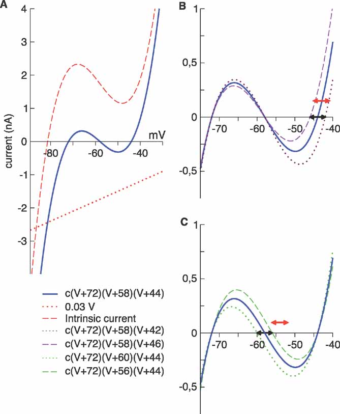
Figure 1. (A) nonlinear membrane current. The combination of a nonlinear intrinsic current, such as a cubic nonlinearlity with a single real root (dashed line) and a linear “external” contribution (dotted line) can give rise to an effective bistability (solid line). In this example, the linear term has an excitatory effect. B-C: bistability and disorder. In both panels, the solid line is the current Inl computed using the mean values of , , and . (B) was given the maximal (dotted line) and minimal (dashed line) values of its distribution; the black segment denotes the corresponding interval, ( - 46, - 42) mV. The threshold of the membrane potential takes values in the interval ( - 45, - 41) mV (red segment). (C) was given the maximal (dashed line) and minimal (dotted line) values of its distribution; the black segment denotes the corresponding interval, ( - 60, - 56) mV. The reset potential takes values in the interval ( - 56, - 52) mV (red segment). In the legend, c is a constant.
In the absence of other currents, Inl(t) induces three fixed points, at the values V1, V2, and V3, which are related but not equal (due to the leak current) to , , and . In the absence of fluctuating currents, the neuron will fire only if V(t) stays in the region above the unstable fixed point at V2 (this requires Vreset to be above this fixed point) and if Vth is less than the upper stable fixed point at V3. If the threshold satisfies Vth > V3, the membrane potential will remain stuck at the value V3. On the other hand, if V is in the region below the unstable fixed point at V2, it will be attracted to the quiescent fixed point at V1. In the network we study, fluctuations produced by both the synaptic currents and the external source of noise Inoise allow the neuron to fire even if its threshold is above the upper fixed point.
Most neuron parameters within the network are distributed stochastically. Because the relationship between the neuron parameters Vreset, Vth, and Vi (or equivalently ) for i = 1, 2, 3 is different for each neuron, most neurons transition from one state to the other with some regularity, but others tend to remain either silent or firing most of the time. Figure 1
B shows the range of ∼V3 (black segment) and Vth (red segment) used in the network. There is a small bias toward neurons with Vth > ∼V3. Similarly, Figure 1
C shows the range used for ∼V2 (black segment) and Vreset (red segment).
Each neuron receives independent noise Inoise consisting of two Poisson trains, one excitatory and one inhibitory. The noise model has four parameters: two unitary conductances (Δgsyn, E and Δgsyn, E) and two rates. This noise is filtered according to Equation (3) through synapses with slow synaptic time constants (i.e., τNMDA and τGABAB).
We have implemented sensory stimulation by the application of a pulse of excitatory conductance to a subpopulation of the excitatory neurons in the network. Minimal stimulation was defined as the minimal conductance of a pulse required to evoke an up state from a down state with high probability.
Parameter Values and Simulations
Most of the results presented were obtained for fixed values of the model parameters, although the results presented in Figure 4 A (see figure caption) and the analysis of the network with zero adaptation conductance are an exception. Otherwise, only the noise term was varied to observe how it affects network activity.
The network contains 4000 neurons of which 17% are inhibitory and the rest excitatory. Each neuron is connected with a probability of 2% to other neurons contained within a disk centered about its location and containing about 31% of the total number of neurons. This results in each neuron, on average, connecting to 25 other neurons. The network size is 50 × 80, with periodic boundary conditions.
All the neurons have a membrane time constant of 20 ms and a refractory time τrefr = 5 ms. Other passive properties are distributed uniformly, and we use a ± notation to indicate the interval within which each parameter falls uniformly. The membrane threshold Vth takes values in the interval - 45 ± 2 mV, the reset potential Vreset in the interval - 55 ± 1 mV, and the leak potential VL in the interval - 68 ± 1 mV. The parameters of the nonlinear current, with conductance measured in units of the leak, are c = 0.03 mV - 2, and the  were chosen as = - 72 ± 2 mV, = - 58 ± 2 mV, and = - 44 ± 2 mV.
All excitatory synapses include both AMPA and NMDA components. On the other hand, we assigned GABAA receptors to 55% and GABAB receptors to 45% of the inhibitory synapses. The synaptic time constants are τAMPA = 2 ms, τNMDA = 100 ms, τGABAA = 10 ms, and τGABAB = 200 ms. Recall that all conductances are measured in units of the leak conductance of excitatory neurons. For excitatory neurons, ΔgE,AMPA = 0.27, ΔgE,NMDA = 0.0495, ΔgE,GABAA = 0.84, ΔgE,GABAB = 0.1848. For inhibitory neurons, ΔgI,AMPA, ΔgI,NMDA = 0.05, ΔgI,GABAA = 0.017, ΔgI,GABAB = 0.017, and gI,L = 1.4. In addition, for excitatory neurons Δga = 0.14, Va = - 80 mV, and τa = 100 ms. The reversal potentials for the inhibition, VGABAB and VGABAA fall uniformly within the intervals - 90 ± 2 mV and - 80 ± 2 mV, respectively. VAMPA and VNMDA are both set to zero.
The parameters of the noise model were varied to study how network behavior was modulated by noise. We started with a network characterized by the following values: Δgsyn,E = 0.09, Δgsyn,I = 0.179 for the conductances and νsyn,E = 66.66 Hz, νsyn,I = 24.31 Hz for the rates. Other networks were obtained by multiplying the inhibitory noise conductance Δgsyn,I by factors that are given in the Results.
We have also considered a network with zero adaptation conductance (Δga = 0). In this case the values of the synaptic conductances were taken as follows: For excitatory neurons, ΔgE,AMPA = 0.20, ΔgE,GABAA = 0.21, ΔgE, GABAB = 0.21. For the inhibitory neurons, ΔgI, AMPA = 0.12, ΔgI, NMDA = 0.025, ΔgI, GABAA = 0.008, ΔgI, GABAB = 0.0085.
The network was stimulated by applying conductance pulses to 17% of the excitatory neurons (either in a localized or in a distributed way) for 10 ms. The size of the pulse for minimal stimulation is gmin ∼ 1 - 1.1. The result of this calibration can be observed in Figure 9 .
For individual neurons the transition from one state to the other was defined to occur at V = - 60 mV, where V is the potential of the neuron. This value separates the two peaks in the membrane potential distribution (see Figure 3 A).
At the network level, the down–up transition was taken at the point where the average membrane potential is equal to the mean of its minimum value in the down state and its peak value in the up state, and a similar criterion was used to define the up–down transition.
Simulation times were typically from a few seconds to 25 seconds, and in some cases up to 100 seconds. Time was divided into bins of size Δt = 0.1 ms. The simulation was done using a computer code written in C and run under the Linux operating system.
Results
Spontaneous Activity
The network has a variety of activity regimes depending on the values of the model parameters. The set of parameter values given in the Methods defines a network that generates spontaneous up states at a rather regular frequency of approximately 0.6 Hz (Figure 2 ). These transitions can be seen most easily in global quantities such as the population rate and average membrane potential (Figures 2 A, B, and E, respectively). The latter can be used as a surrogate for the local field potential. The phenomenon is quite robust, and the appearance of a signal in global quantities implies that a large population of neurons transition between up and down states synchronously (Figure 2 D). However, the up states are not identical, nor are the times that the network spends in these states always the same. This indicates that the state of the network at the onset of these up states is variable.
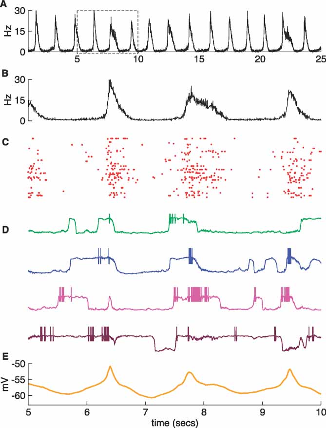
Figure 2. A regular network. (A) Population rate over 25 seconds; the other traces correspond to the time interval from t = 5 to t = 10 seconds (box). (B) Expanded population rate. (C) Rastergram (100 neurons). (D) Membrane potential of 4 neurons. (E) Average membrane potential. The mean rate in the up state is 6–7 Hz for the excitatory neurons and 13–14 Hz for the inhibitory neurons.
Traces of the membrane potential of individual neurons (Figure 2 D) show less regular up–down dynamics than global quantities. Even when the synchrony is evident in the average membrane potential, there is some variability in the timing of the transitions for different neurons. In these respects, this example resembles the observations by Lampl et al. (1999) in primary visual cortex that the correlations of the membrane potential of pairs of nearby neurons are weaker than those observed, for example, in slow-wave sleep, and that even the degree of subthreshold synchrony exhibited by a given pair can change with time. However, the model can support more correlated populations. Figure 4 A presents an example in which the distribution of firing thresholds and some of the unitary conductances were changed to obtain more synchronous transitions.
The four neurons shown in Figure 2 D were selected to illustrate the different membrane potential distributions displayed in Figure 3 A. These distributions are all bimodal, but they show different splits between the two peaks. For the neurons shown in the two upper panels of Figure 2 D, corresponding to the upper two panels in Figure 3 A, both peaks are comparable, but the other two neurons, shown in the lower panels of these figures, remain in the down or in the up state most of the time.
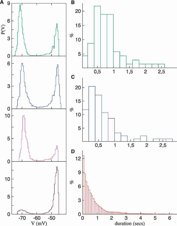
Figure 3. Characterization of the slow fluctuations of the regular network. (A) Potential distributions of the four neurons shown in Figure 2 D. Note that the neuron shown at the bottom (brown line) stays most of the time in the up state. (B–C) Histograms for the duration of the up states of two bimodal neurons. The simulation time was 100 seconds. (D) Histogram of the duration of the up states computed from all the neurons in the network.
Figures 3 B and C present histograms of the duration of the up states for two neurons that have bimodal membrane potential distributions. The distribution for the duration of up states across the entire network is shown in Figure 3 D. Although bimodal neurons have distributions concentrated around a preferred duration, as in (Stern et al., 1998 ), the data taken over the whole network has a more varied distribution with a tail reaching durations of a few seconds (Figure 3 D). (Cossart et al., 2003 ) have observed an even longer tail including durations of about 10 seconds. Although we have not tried to reproduce this observation, it is conceivable that a proper choice of the distribution of neuron properties could generate a subpopulation of neurons with longer up states.
To illustrate the evolution of the synaptic conductances, we plotted the network average of the inhibitory conductance versus the corresponding average of the excitatory conductance (Figure 4 B). In this plot, time advances counter-clockwise along the lines. The first second of the simulation has been included in this figure, resulting in the initial transient seen as the line departing from the origin. After this transient, the plot consists of a series of ellipses each describing the evolution of the synaptic conductances during one transition to the up state and back to the down state. The excitatory conductance is the first to grow followed by inhibition until the latter becomes strong enough causing the excitatory conductance to decrease.
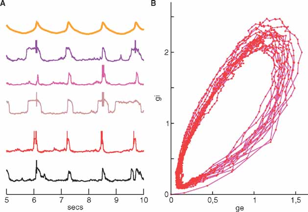
Figure 4. (A) A more synchronous network. The distribution of the membrane threshold and some of the unitary conductances have been changed to induce more synchronous transitions. The synaptic inhibitory conductances were 70% of those described in the Methods. In addition, Δgsyn,I = 0.197 and Vth = - 45.5±2. Note the sharp increase in the average membrane potential (top trace) correlated with neuron firing, which is similar to the LFP observed in (Destexhe et al., 1999 ). (B) Evolution of the average conductances in the regular network of Figures 2 and 3 . The average inhibitory synaptic conductance gi versus the average excitatory synaptic conductance ge, with time as an implicit parameter. The red dots indicate the data at the sampling times. Both conductances increase as the network makes a transition from the down to the up state.
The transition from the down to the up state results from the interaction between the nonlinear property of the neurons and synaptic activity in the population. When the network is in the down state, most, but not all, of the neurons are silent. The activity of the small number of active neurons (plus possible current fluctuations coming from the noise) propagates through the network causing neurons to transit to the up state. Eventually, a large number of neurons make this transition, and the population rate increases. During the transition to the up state, the excitatory conductances are the first to increase, but they are soon followed by the inhibitory ones (Figure 4 B). After some time, inhibition becomes strong enough to destabilize the up state of individual neurons, and eventually the network returns to the down state. Most of the inhibitory neurons do not fire in the down state. Rather, the network is maintained in this state because of a lack of excitation (as observed in (Timofeev et al., 2001 )) and due to the effective bistability of the neurons.
Transitions from the up to the down state can also be interpreted in terms of an oscillatory property of networks of normal IF neurons. When our network is in the up state, it behaves like a network of IF neurons kept depolarized at a potential approximately equal to the average potential of the up state. It has been shown that synaptic delays introduce an oscillating mode in such networks (Brunel and Wang, 2003 ). For normal IF neurons, the population rate oscillates in complete cycles, with inhibition following excitation, at a frequency determined by the synaptic time constants. In our model, the neurons start to fall into the down state as the network approaches the negative phase of the oscillation, so the cycle is interrupted. Whereas the time the network stays in the up state is mainly determined by the mechanism just described, the time that it spends in the down state is defined by different factors; the number of neurons firing during the down state, the distribution of neuron parameters, and the connectivity of the network.
The termination mechanism described above does not require neuronal adaptation. This was checked by removing all adaptation, using the values of the synaptic conductances given in the Methods section. In the absence of adaptation, the transition to an up state starts with a rise of the excitatory conductance followed by inhibition. When the inhibition becomes sufficiently strong, the network goes back to a down state. Adaptation was included in the model for the sake of biological realism, but it is not an essential element of the up-down dynamics of the model.
Noise Modulation
The dynamics of up–down transitions can be modulated by changing the relative strength of the excitatory and inhibitory components of the noise. We limited this analysis to changes of the inhibitory unitary conductance of the noise, Δgsyn,I, leaving the other three parameters in the noise model fixed. Changing the excitatory unitary conductance yields qualitatively similar results. Taking the network in Figures 2 and 3 as the starting point, we first look at the effect of reducing Δgsyn,I. Figure 5 presents a network in which this was reduced by 15%. The top trace is the population rate during 25 seconds, and the rest of the figure is an expansion of the time interval between 5 and 10 seconds. Another 5 seconds time interval (20–25 seconds) is shown in Figure 6 . Decreasing the inhibitory component of the noise makes the network transitions more irregular. For example, the network makes a single transition to the down state from 5–10 seconds, but it exhibits four up states of different durations during the interval from 20–25 seconds.
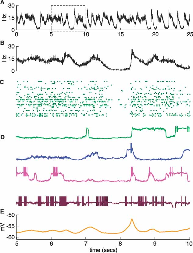
Figure 5. A more irregular network I. The inhibitory conductance of the noise model was decreased by 15% with respect to that of the regular network in Figures 2 and 3 . The traces are shown with the same convention as in Figure 2 , and the four neurons in D are the same as those in Figure 2 D. The expanded box and panels B–E show the interval between 5 and 10 seconds during the simulation. A synchonous transition occurs after t = 8 seconds.
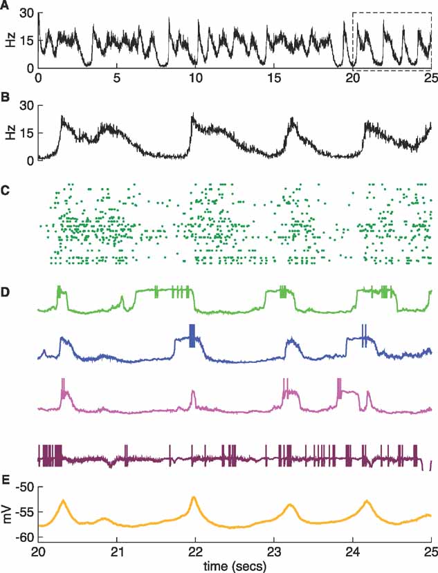
Figure 6. A more irregular network II. Same as Figure 5 , but now the expanded box and panels B–E show the last five seconds of the simulation. Four up-state transitions occur during this time.
If the inhibitory noise conductance is decreased even more, the system eventually reaches a regime in which neurons either fire tonically or become inactive. Setting Δgsyn,I to 50% of its value in the regular network produces the active network shown in Figure 7 . This network is asynchronous, the average membrane potential is below the value of the mean potential of the up state (Figure 7 B), and a subpopulation of neurons in the network fire continuously while the others tend to stay in the down state most of the time. Three of the neurons described in Figure 2 have greatly reduced activity, while the other has become more active (compare the traces in Figure 7 C with those in Figure 2 D). Another relevant feature of this regime is that the average inhibitory synaptic conductance is larger than the excitatory (Figure 7 D). These two features, namely the existence of a population of silent neurons and the dominance of inhibition, have been observed in a recent experiment during the activated state characteristic of cortical networks in awake animals (Rudolph et al., 2007 ).
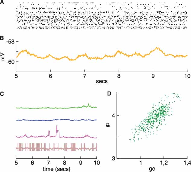
Figure 7. An active network. The inhibitory conductance of the noise was reduced to 50% of its value in the regular network. Neurons tend either to fire tonically or be inactive. (A) Raster. (B) Average membrane potential. (C) Membrane potential traces for the same neurons as in Figures 2 , 5 , and 6 . (D): Evolution of the average conductances. The average inhibitory conductance is now larger than the excitatory in agreement with experimental observations (Rudolph et al., 2007 ).
The transition from the regular network to the active network shown in Figure 7 is reminiscent of the transition from slow-wave sleep oscillations to the activated state (Steriade et al., 2001 ; Timofeev et al., 2001 ), controlled by neuromodulators (Steriade and McCarley, 1990 ). In particular, release of acetylcholine reduces or blocks potassium conductances (McCormick, 1992 ; Steriade et al., 1993 ) leading to a greater excitability of cortical neurons. This issue has been considered in biophysically detailed models by blocking resting potassium conductances (Bazhenov et al., 2002 ) or reducing other potassium conductances (Compte et al., 2003 ). The fact that the network becomes dominated by inhibition and splits into a firing and a silent population after the transition to the tonically active state was not apparent in those models. Although we have controlled the network dynamics by changes in the noise parameters, similar results could be obtained if the neuron excitability were increased by other means.
If Δgsyn,I is made 10% larger than its value in the regular network, the network becomes more tied to the down state (Figure 8 ). Although there is still some spiking and individual neurons still transition between the two states, the coherence has been lost, as evident in the trace of the average membrane potential (Figure 8 C) and in the values of the average synaptic conductances which are about a factor 10 smaller than in the initial network (Figure 8 F). In the following section, we address the issue of the excitability of this network. As we will see, stimulating the system, while it is in this regime evokes up states similar to those generated spontaneously in the regular network.
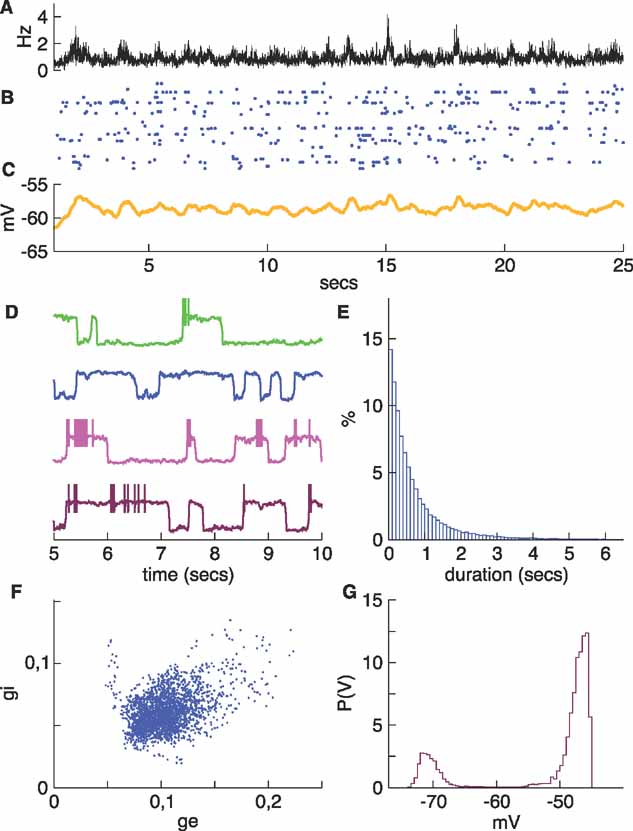
Figure 8. A rather silent network. The inhibitory conductance of the noise was increased by 10%. Neurons still make transitions between up and down states, but the synchrony is lost. (A) Average firing rate. (B) Raster. (C) Average membrane potential. (D) Sample membrane potential traces for the same four neurons shown in previous figures. The bottom trace (brown), which corresponds to the neuron that stayed mostly in the up state in the more active networks (brown traces in Figures 2 , 5 and 7 ) now makes transitions and develops a bimodal potential (panel G). (E) Histogram of up state durations. These are shorter than in more active networks. (F) Evolution of the average conductances, which are much smaller than in the previous networks. There is no longer any structure in the conductance plane.
Sensory Stimulation
Sensory stimulation can evoke responses similar to the up state seen during spontaneous activity (Petersen et al., 2003 ). Up states can also be evoked in slices by stimulating thalamic fibers (MacLean et al., 2005 ). The activity patterns produced in this way have several similarities to those generated spontaneously. The response of barrel cortex neurons to sensory stimulation was seen to depend on whether it is applied during an up or a down state of the recorded neuron (Petersen et al., 2003 ). Electric stimulation of the thalamus gives a similar result (Sachdev et al., 2004 ).
To study these issues within our model, we first considered whether stimulation of the silent network of Figure 8 is able to evoke up states with properties similar to those seen in the spontaneous activity of the more regular network of Figure 2 . In a second part of our analysis, we stimulated the regular network either during an up or a down state and compared the spiking responses. Up and down states are defined for this purpose using the average membrane potential, which is our surrogate for the local field potential, a global quantity that well characterizes the state of the network. Notice that this procedure is different from what is normally done in experiments, where the stimulus is applied during the up or the down state of the recorded neuron rather than the network (Petersen et al., 2003 ). If the synchrony of the transitions is strong, there should not be much difference between these two procedures. However if it is not, as in (Lampl et al., 1999 ), it seems more sensible to stimulate during the up or the down states defined at the population level because, in this way, the time of application is correlated with a specific network state.
We first stimulated the silent network of Figure 8 , which is in a regime corresponding to a down state, by applying minimal conductance pulses every 2 seconds. This evoked up states most of the time (Figure 9 ). Note that during the 25 seconds of this simulation the stimulus failed to evoke an up state only once (at t = 8 seconds in Figures 9 A–C), and, even in this case, the trace of the average potential (Figure 9 C) shows that many neurons in the network made a transition to that state. It is likely that the network transition was not completed because the stimulus failed to propagate and recruit a sufficient number of neurons. Because each time that a pulse is applied the state of the network is different, the temporal profiles of global quantities are variable. A notable difference from the spontaneous up state is the existence of two peaks in the population rate (Figure 9 A). Presumably, the first peak is due to the response of the neurons receiving a direct stimulation, and the time between the peaks corresponds to the time needed for the propagation of the evoked activity through the network until a substantial number of neurons also responds to the stimulus. A response with two peaks is also present in experiments (see Figure 5 in (Petersen et al., 2003 )).
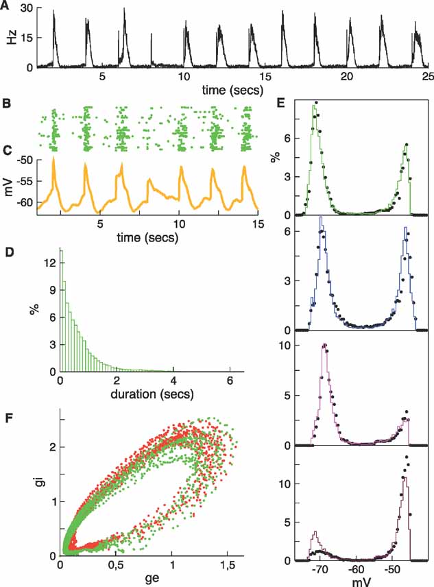
Figure 9. Periodic sensory stimulation of the silent network and characterization of the evoked slow fluctuations. (A) The population rate of the silent network when it is minimally stimulated every 2 seconds. During the 25 seconds of this simulation the stimulus failed to evoke an up state only once (at t = 8 seconds). (B) Raster for the first 15 seconds of the simulation. (C) Average potential. (D) Histogram of the durations of the up states. (E) Membrane potential histograms for the same four neurons shown previously. The black dots show data from Figure 3 . (F) Evolution of the average conductances is indicated by the green dots. For comparison, the red dots are data from Figure 4 B.
There is considerable similarity between the regular (Figure 2 ) and the stimulated silent (Figure 9 ) networks, even when the stimulation period is only roughly equal to the average spontaneous up–down state period, and when the spontaneously evoked up states are not strictly periodic. To facilitate comparison, the black dots shown with the potential distributions (Figure 9 >E) and the red dots in the conductance plane (Figure 9 F) are results from Figure 2 .
In the example of Figure 9 , the period of the stimulation was long enough to allow the network to recover back to the silent (down) state. If the stimulation frequency is increased, the second pulse can occur while the network is in a state close to the up state evoked by the first pulse, and the response can change dramatically. The effect of stimulation frequency on the generation of up states is described in Figure 10 . The traces and rastergram at the top correspond to a single pulse applied at t = 2 s to the silent network shown in Figure 8 . The next four rows present the result of stimulating with different frequencies; pulses have been applied every 1.3 second, 1.4 second, 100 ms, and 50 ms (from top to bottom). In the first case, the second pulse fails to evoke an up state because the network falls into the down state and there is little excitation. Although a subpopulation of neurons fires most of the time, there is a delay before the activity spreads to enough neurons to produce a synchronous transition to the up state. The trace of the average potential (Figure 10 , right column) shows that, although many neurons made the transition, the excitation did not extend to a large portion of the network. In the example of the third row of Figure 10 , the second pulse is applied after 1.4 seconds, and the extra 0.1 seconds provides enough time for the network to gather sufficient excitation to produce a second up state. Even so, it takes a rather long time for the activity to spread across the network and evoke a global up state. Had we applied the second pulse a little later (e.g., after 1.5 seconds), the transition would have been faster (data not shown). The third pulse in this example comes too soon after the preceding up state, so its effect on both the firing and the subthreshold responses is small, and again it fails to evoke a synchronous transition. An example at an even lower frequency has already been seen in Figure 9 where, as we discussed, up states are evoked with high probability. On the other hand, as the frequencies become higher, the second pulse arrives on the decaying phase of the up state and its effect is minute. As an example, we show the responses for a stimulation frequency of 10 Hz (fourth row of Figure 10 ). The effect of each pulse is small, but the frequency is relatively high so the effect of consecutive pulses accumulates and up states are evoked sooner than in the previous examples. In the final example, a train of pulses at 20 Hz is applied for more than 2 seconds (Figure 10 , bottom panel). At this frequency, the increase of the average potential evoked by a pulse roughly compensates its decay, and the network stays in a depolarized state intermediately between the down and the up states.
The previous discussion shows that the response to sensory stimulation depends on how deeply into the up or down state the network is at the time of the application of a pulse. After a transition from an up to a down state, the network has to recover before being able to evoke another up state. This recovery occurs through the neurons that are able to continue firing most of the time. Too close to the previous up state, there is still some inhibition that prevents these neurons from firing, but after some time the network arrives in its down state (where there is no appreciable inhibition), and the active neurons increase their firing and put the network into a more responsive state.
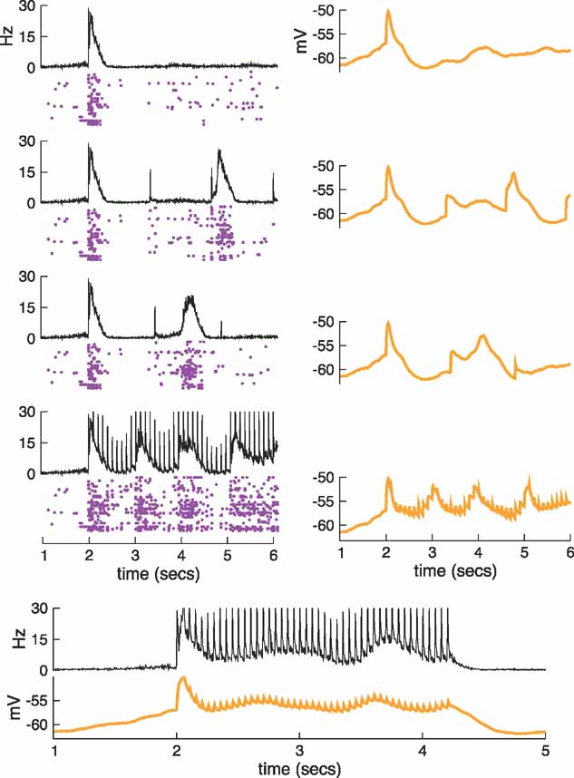
Figure 10. The effect of stimulation frequency on the generation of up states. In the top row, a single pulse has been applied. In the following rows, from top to bottom, the stimulus has frequencies of 0.77, 0.71, 10 and, in the bottom panels, 20 Hz. Each of the top four rows contains the population rate and the rastergram (left column) and the average membrane potential (right column). At the bottom, the population rate and average membrane potential are stack to allow for a greater time resolution. In the second row, the second pulse at 0.77 Hz fails to generate an up state. In the third row, the second pulse at 0.71 Hz succeeds in evoking an up state. Comparison of these traces with those obtained at 0.5 Hz in Figure 9 shows that the activity propagates more slowly (the second peak in the population rate occurs after a longer time). For stimulation at 10 Hz and above (fourth row and bottom), the membrane remains depolarized during all of the stimulation time.
The response to sensory stimulation is much larger if a pulse arrives when the network is in the excitable phase of its down state than when it is in an evoked up state. On may wonder whether the same is true when the stimulation is applied to a network capable of generating spontaneous transitions, such as the regular network described in Figures 2 and 3 . The result of this analysis is shown qualitatively in Figures 11 and 12 and more quantitatively in Figures 12 D. The left column in Figures 11 shows three spontaneous up states. To exhibit the dependence of the response on the spontaneous fluctuations, we stimulated on the second up state (at t = 3.4 second) and compared the response with the responses to stimulation in two down states, at t = 2.8 and 4.0 seconds.
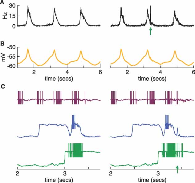
Figure 11. Stimulation during an up state of the regular network. Left: Regular network showing spontaneous regular transitions to the up state (same network as in Figures 2 and 3 ). Right: Stimulating during an up state of the network at t = 3.4 seconds. The stimulus has little effect on the network when applied during the up state. At the bottom of this figure we show the effect of the stimulus on the membrane potential traces of three neurons. The arrow indicates the stimulation time.
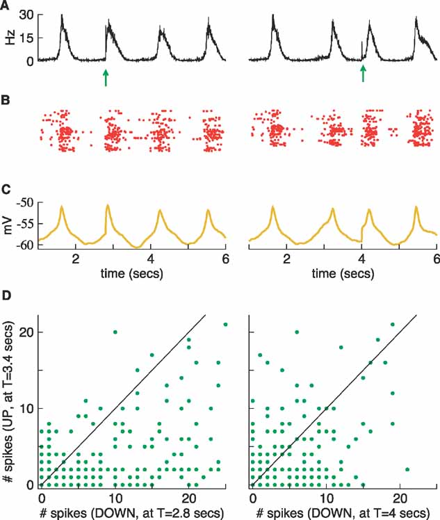
Figure 12. Dependence of the spiking responses on network state. This is the same network as in Figure 11 , but now the stimulus is applied during the first down state at t = 2.8 seconds (left) and during the second down state at t = 4 s (right). (A) Population rates. (B) Rastergrams. (C) Average membrane potentials. (D) These graphs compare the number of spikes produced by individual neurons when the network was stimulated during the down states (as in the upper panels) compared to those produced by stimulating during the up state (as in Figure 11 , right). Spikes are counted within a time window of 200 ms following the application of the stimulus.
In the right column of Figure 11 , we see that stimulating during the spontaneous up state has little effect. As the traces of the population rate and the average membrane potential indicate, the effect of the stimulation is localized in time. Shortly after the stimulation, these traces continue their temporal course without undergoing any relevant change, and the third spontaneous up state remains almost unperturbed.
The stimulus has a very different effect when it is applied during a down state (Figure 12 A–C). In the two cases presented here (stimulus applied during the first (left column) and during the second (right column) down states), a new up state is evoked and the next spontaneous state is pushed forward in time. The increment in the number of spikes is clearly larger under stimulation during the down than during the up states. Some experimental observations in rats seem to indicate that the spiking response is higher in absolute terms as well (Petersen et al., 2003 ), although in cats the opposite result is obtained (Haider et al., 2007 ). We studied this issue in our model by plotting the number of spikes produced by individual neurons under the conditions used in Figure 11 (right column) against the number of spikes produced under stimulation in one of two down states. The result of this test is shown in Figure 12 D. While the stimulation during the first down state (Figure 12 , left column) agrees with the experimental observation in (Petersen et al., 2003 ), exhibiting a much larger response for stimulation in the down state, stimulation during the second down state (Figure 12 , right column) reveals a more balanced situation. The explanation for this difference is again the different state of the network at these two points. At t = 4 seconds, the average potential is almost at its lowest point in the second down state (Figure 11 , left column) and the network is almost as hyperpolarized as it ever is during spontaneous behavior. In contrast, at t = 2.8 seconds the network is already naturally evolving toward the next spontaneous up state, a fact that is clearly seen in the average potential although it is less evident in the population activity (see Figure 11 , left column). At this point the network is ready to fire, but it is not yet doing so and, as a result, the arrival of the stimulus has a strong impact. This is also why the peak of the average potential is reached sooner in this case.
In contrast with the case of evoked up states, the network with spontaneous fluctuations has an excitable phase, located at the beginning of the up state. When the response to stimulation in this region (e.g., at t = 3.2 seconds in Figure 11 ) is compared with the response to stimulation in a down state (e.g., at t = 4 seconds) one finds that, in absolute terms, the response in the up state is higher than that in the down state.
We now ask which response is stronger when the stimulation time is chosen randomly. Because both the up and the down states have an excitable phase and a less excitable phase, the answer to this issue depends on their relative durations. Given the variability observed in the time course of the average membrane potential (present even in our regular network), a careful analysis is required. We have run repeated simulations of the regular network, stimulating at different times. The stimulation period was 50 ms and the longest simulation had a duration of 25 seconds. After this, a set of neurons (either the whole network, those receiving the stimulus directly or a set of randomly chosen neurons) was selected, and for each neuron a stimulation time in an up state and another in a down state was chosen, also at random. For the regular network, the response to stimulation in the up state was larger. For example, when the test described here was done over the whole network, the spiking response (total number of spikes) during the up states was about 1.55 times larger than during the down states.
This result is in agreement with experimental observations in the cat (Haider et al., 2007 ). It holds regardless of the degree of localization of the stimulus. However, because a change in the values of the conductances and other model parameters can change the regularity of the transitions and the relative size of the excitable phases of the up and down states, this model could, in principle, exhibit regimes where the response to stimulation in the down state is the stronger.
Discussion
We have presented a simple model that is able to reproduce some of the most important properties of the up–down dynamics observed in cortical networks. The model has two main features: the interaction between a nonlinear intrinsic property of the neurons with the synaptic activity and the heterogeneity in the neuron parameters. The first provides two stable states and fluctuations that facilitate the transitions between them, whereas the second generates a subpopulation of neurons that spontaneously reactivates the network after it returns to a down state. Along with a regime exhibiting spontaneous synchronous transitions between up and down states, the model has irregular, active, and inactive states, and the network can transit between them under the control of some of the model parameters. The response of the network to a stimulus depends on the state at the moment of the stimulation, with a higher response occurring when the network is in the down state.
The Up–down Dynamics
In our model, the transition from the down to the up network states occurs because of the activity of neurons that remain in their up state most of the time. A similar phenomenon occurs in more detailed biophysical models (Compte et al., 2003 ; Hill and Tononi, 2005 ; Kang et al., 2004 ). In (Kang et al., 2004 ), the activity of a subpopulation of pacemaker neurons is based on the Ih current in combination with a low threshold Ca2+ current. In (Hill and Tononi, 2005 ) an Ih current is used in combination with a persistent sodium current, which activates some neurons and leads the whole network into the active state. Other modeling studies proposed a mechanism based on the presence of spike-independent minis during the inactivated network state that can add up to produce a transition from the down to the up state (Bazhenov et al., 2002 ; Timofeev et al., 2000 ).
The mechanism for the termination of the up state in our model is different from those proposed in other modeling studies. In our model, the up state is terminated by a network oscillatory mechanism in which the inhibition following excitation destabilized the up state causing the network to return to a down state. The time scale of this process, which determines the average duration of the up states, depends on the synaptic time constants and can be controlled by the type of synaptic receptors used in the model. For example, the frequency of the slow oscillation in the regular regime increases to about 4 Hz, namely in the delta range, if only fast excitation and inhibition (AMPA and GABAA) are included (data not shown).
Response to Sensory Stimulation
Large fluctuations of the membrane potential can affect the response to sensory stimulation. In rat barrel cortex, if the stimulus occurs while the potential is in an up state both subthreshold and spiking responses are suppressed relative to the response to a stimulus arriving during a down state. Possible sources of this phenomenon include network and neuronal factors. The strong network activity during the up state increases the conductance leading to shunting of the EPSPs. Short-term depression could also have a suppressive role because it acts during the up state (a model of the up-down dynamics based on synaptic short-term depression was proposed in (Holcman and Tsodyks, 2006 ). In addition, differences in the strength of the driving forces between the two states and in the value of the threshold for action potentials could also contribute to the different responses (Sachdev et al., 2004 ).
In cats, the response in the up state is the strongest (Haider et al., 2007 ). The model reproduces this phenomenon. In the model, the bias in the strength of the response towards either the down or the up state is due to a difference in the relative sizes of the excitable phases of those states. In turn, this difference depends on the strength of the synaptic conductances. We have studied this issue only in our regular network, finding that, in this regard, it predicts a response similar to the findings in cats. It is an open question whether the model with different parameter values can also explain the findings in rat barrel cortex or if it is necessary to include effects such as short-term depression, which was not considered in the model.
Conclusions
In summary, a network model built from IF neurons augmented with a nonlinear membrane current and connected sparsely through slow and fast excitatory and inhibitory synaptic conductances can capture much of the phenomenology of down and up states in cortical slices and in vivo recordings. The model suggests that an examination for bistable properties that arise when network effects interact with intrinsic conductances would be an interesting way to explore experimentally what appears to be an important element of up–down state transitions.
Conflict of Interest Statement
The authors declare that the research was conducted is the absence of any commercial or financial relationships that should be construed as a potential conflict of interest.
Acknowledgments
We are extremely grateful to Rafael Yuste for essential insights and guidance in the construction and testing of this model. N. P. wishes to thank the Center for Theoretical Neuroscience at Columbia University for their hospitality during his visit. This research was supported by the Swartz Foundation and by an NIH Director's Pioneer Award, part of the NIH Roadmap for Medical Research, through grant number 5-DP1-OD114-02.
References
Amzica, F., and Steriade, M. 1995. Short- and long-range neuronal synchronization of the slow (<1Hz) cortical oscillation. J. Neurophysiol. 73, 20-38.
Anderson, J., Lampl, I., Reichova, I., Carandini, M., and Ferster, D. 2000. Stimulus dependence of two-state fluctuations of membrane potential in cat visual cortex. Nat. Neurosci. 3, 617-621.
Arieli, A., Sterkin, A., Grinvald, A., and Aertsen, Ad. 1996. Dynamics of ongoing activity: explanation of the large variability in evoked cortical responses. Science 273, 1868-1871.
Bazhenov, M., Timofeev, I., Steriade, M., and Sejnowski, T. J. 2002. Model of Thalamocortical Slow-Wave Sleep Oscillations and Transitions to Activated States. J. Neurosci. 22, 8691-8704.
Brunel, N., and Wang, X.-J. 2003. What determines the frequency of fast network oscillations with irregular neural discharges? I. synaptic dynamics and excitation Inhibition balance. J. Neurophysiol. 90, 415-430.
Compte, A., SanchezVives, M. V., McCormick, D. A., and Wang, X.-J. 2003. Cellular and Network Mechanisms of Slow Oscillatory Activity (<1Hz) and Wave Propagations in a Cortical Network Model. J. Neurophysiol. 89, 2707-2725.
Cossart, R., Aronov, D., and Yuste, R. 2003. Attractor dynamics of network UP states in the neocortex. Nature 423, 283-288.
Crunelli, V., Toth, T. I., Cope, D. W., Blethyn, K., and Hughes, S. W. 2005. The ‘window’ T-type calcium current in brain dynamics of different behavioural states. J. Physiol. (Lond) 562, 121-129.
CrossRef Full Text | /a>
Destexhe, A., Contreras, D., and Steriade, M. 1999. Spatiotemporal analysis of local field potentials and unit discharges in cat cerebral cortex during natural wake and sleep states. J. Neurosci. 19, 4595-4608.
Frohlich, F., Bazhenov, M., Timofeev, I., Steriade, M., and Sejnowski, T. J. 2006. Slow state transitions of sustained neural oscillations by activity-dependent modulation of intrinsic excitability. J. Neurosci. 26, 6153-6162.
Haider, B., Duque, A., Hasenstaub, A. R., Yu, Y., and McCormick, D. A. 2007. Enhancement of visual responsiveness by spontaneous local network activity in vivo. J. Neurophysiol. 97, 4186-4202.
Hill, S., and Tononi, G. 2005. Modeling sleep and wakefulness in the thalamocortical system. J. Neurophysiol. 93, 1671-1698.
Holcman, D., and Tsodyks, M. 2006. The Emergence of Up and Down States in Cortical Networks. PLoS Comput. Biol. 2, e23.
Kang, S., Kitano, K., and Fukai, T. 2004. Selforganized two-state membrane potential transitions in a network of realistically modeled cortical neurons. Neural Netw. 17, 307-312.
Lampl, I., Reichova, I., and Ferster, D. 1999. Synchronous Membrane Potential Fluctuations in Neurons of the Cat Visual Cortex, Neuron 22, 361-374.
MacLean, J. N., Watson, B. O., and Yuste, R. 2005. Internal Dynamics determine the cortical response to thalamic stimulation. Neuron 48, 811-823.
Mao, B. Q., Hamzei-Sichani, F., Aronov, D., Fromke, R. C., and Yuste, R. 2001. Dynamics of spontaneous activity in neocortical slices. Neuron 32, 883-898.
McCormick, D. A. 1992. Neurotransmitter actions in the thalamus and cerebral cortex and their role in neuromodulation and thalamocortical activity. Prog. Neurobiol. 39, 337-388.
Metherate, R., and Ashe, J. H. 1993. Ionic flux contributions to neocortical slow waves and nucleus basalis- mediated activation: whole-cell recordings in vivo. J. Neurosci. 13, 5312-5323.
Petersen, C. C. H., Hahn, T. T. G., Mehta, M., Grin-vald, A., and Sakmann, B. 2003. Interaction of sensory responses with spontaneous depolarization in layer 2/3 barrel cortex. PNAS 100, 13638-13643.
Rudolph, M., Pospischil, M., Timofeev, I., Destexhe, A. 2007 Inhibition determines membrane potential dynamics and controls action potential generation in awake and sleeping cat cortex. J. Neurosci.
Sachdev, R. N. S., Ebner, F. F., and Wilson, C. J. 2004. Effect of subthreshold up and down states on the whisker evoked response in somatosensory cortex. J. Neurophysiol. 92, 3511-3521.
Sanchez-Vives, M. V., and McCormick, D. A. 2000. Cellular and network mechanisms of rhythmic recurrent activity in neocortex. Nat. Neurosci. 3, 1027-1034.
Seamans, J. K., Nogueira, L., and Lavin, A. 2003. Synaptic basis of persistent activity in prefrontal cortex in vivo and in organ-otypic cultures. Cereb. Cortex 13, 1242-1250.
Steriade, M., and McCarley, R. W. 1993. Brainstem control of wakefulness and sleep (New York, Plenum).
Steriade, M., Nunez, A., and Amzica, F. 1990. A novel slow (<1Hz) oscillation of neocortical neurons in vivo: depolarizing and hyperpolarizing components, J. Neurosci. 13, 3252-3265.
Steriade, M., Nunez, A., and Amzica, F. 1993. Intracellular analysis of relations between the slow (<1Hz) neocortical oscillation and other sleep rhythms of the electroencephalogram. J. Neurosci. 13, 3266-3283.
Steriade, M., McCormick, D. A., and Sejnowski, T. J. 1993. Thalamocortical oscillations in the sleeping and aroused brain. Science 262, 679-685.
Steriade, M., Timofeev, I., and Grenier, F. 2001. Natural waking and sleep states: a view from inside neocortical neurons. J. Neurophysiol. 85, 1969-1985.
Stern, E. A., Jaeger, D., and Wilson, C. J. 1998. Membrane potential synchrony of simultaneously recorded striatal spiny neurons in vivo. Nature 394, 475-478.
Timofeev, I., Grenier, F., Bazhenov, M., Sejnowski, T. J., and Steriade, M. 2000. Origin of slow cortical oscillations in deafferented cortical slabs. Cereb. Cortex 10, 1185-1199.
Timofeev, I., Grenier, F., and Steriade, M. 2001. Disfacilitation and active inhibition in the neocortex during the natural sleep-wake cycle: An intracellular study. PNAS 98, 1924-1929.
Volgushev, M., Chauvette, S., Mukovski, M., and Timofeev, I. 2006. Precise long-range synchronization of activity and silence in neocortical neurons during slow-wave sleep, J. Neurosci. 26, 5665-5672.
Wilson, C. J., and Groves, P. M. 1981. Spontaneous firing patterns of identified spiny neurons in the rat neostriatum. Brain Res. 220, 67-80.
Wilson, C.J., and Kawaguchi, Y. 1996. The origins of two-state spontaneous membrane potential fluctuations of neostriatal spiny neurons. J. Neurosci. 16, 2397-2410.
Keywords: neuronal modeling, cortical dynamics, cortical network, up-down state transitions
Citation: Néstor Parga and Larry F. Abbott (2007). Network model of spontaneous activity exhibiting synchronous transitions between up and down states. Front. Neurosci. 1: 1. 57-66. doi: 10.3389/neuro.01/1.1.004.2007
Received: 15 August 2007; Paper pending published: 01 September 2007;
Accepted: 01 September 2007;
Published online: 15 October 2007.
Edited by:
Idan Segev, Hebrew University, IsraelReviewed by:
Misha Tsodyks, Department of Neurobiology, Weizman Institute of Science, Israel; Albert Compte, Instituto de Neurociencias, University Miguel Hernandez, SpainCopyright: © 2007 Parga and Abbott. This is an open-access article subject to an exclusive license agreement between the authors and the Frontiers Research Foundation, which permits unrestricted use, distribution, and reproduction in any medium, provided the original authors and source are credited.
*Correspondence: Center for Neurobiology and Behavior, Kolb Research Annex, Rm 759, 1051 Riverside Drive, New York, NY 10032, USA. e-mail: lfa2103@columbia.edu