Optimal temporal risk assessment
- 1 Department of Psychology, Koç University, Istanbul, Turkey
- 2 Princeton Neuroscience Institute, Princeton University, Princeton, NJ, USA
- 3 Department of Psychology, Brown University, Providence, RI, USA
- 4 Department of Psychology, Princeton University, Princeton, NJ, USA
- 5 Program in Applied and Computational Mathematics, Princeton University, Princeton, NJ, USA
- 6 Department of Mechanical and Aerospace Engineering, Princeton University, Princeton, NJ, USA
Time is an essential feature of most decisions, because the reward earned from decisions frequently depends on the temporal statistics of the environment (e.g., on whether decisions must be made under deadlines). Accordingly, evolution appears to have favored a mechanism that predicts intervals in the seconds to minutes range with high accuracy on average, but significant variability from trial to trial. Importantly, the subjective sense of time that results is sufficiently imprecise that maximizing rewards in decision-making can require substantial behavioral adjustments (e.g., accumulating less evidence for a decision in order to beat a deadline). Reward maximization in many daily decisions therefore requires optimal temporal risk assessment. Here, we review the temporal decision-making literature, conduct secondary analyses of relevant published datasets, and analyze the results of a new experiment. The paper is organized in three parts. In the first part, we review literature and analyze existing data suggesting that animals take account of their inherent behavioral variability (their “endogenous timing uncertainty”) in temporal decision-making. In the second part, we review literature that quantitatively demonstrates nearly optimal temporal risk assessment with sub-second and supra-second intervals using perceptual tasks (with humans and mice) and motor timing tasks (with humans). We supplement this section with original research that tested human and rat performance on a task that requires finding the optimal balance between two time-dependent quantities for reward maximization. This optimal balance in turn depends on the level of timing uncertainty. Corroborating the reviewed literature, humans and rats exhibited nearly optimal temporal risk assessment in this task. In the third section, we discuss the role of timing uncertainty in reward maximization in two-choice perceptual decision-making tasks and review literature that implicates timing uncertainty as an important factor in performance quality. Together, these studies strongly support the hypothesis that animals take normative account of their endogenous timing uncertainty. By incorporating the psychophysics of interval timing into the study of reward maximization, our approach bridges empirical and theoretical gaps between the interval timing and decision-making literatures.
Introduction
Evolution appears to have favored at least two well-regulated neurobiological time-keeping mechanisms that are shared by many organisms. One of these mechanisms, circadian timing, captures periods with approximately 24-h cycles. Many events in nature, on the other hand, are non-periodic, and capturing their temporal structure requires a flexible time-keeping apparatus that can be started and stopped as required. To that end, a stopwatch-like mechanism enables many organisms, with high accuracy but limited precision, to time intervals between arbitrary events that range from seconds to minutes. This ability is referred to as interval timing.
Timing intervals allows organisms to organize their relevant activities around critical times (Drew et al., 2005), keep track of reward rates (RRs; Gallistel et al., 2007), or prefer rewards that occur after a short rather than a long delay (Gibbon and Church, 1981; Cui, 2011). Importantly, these apparently simple time-dependent decisions and inferences are inevitably made under endogenous timing uncertainty, and thus entail temporal risk assessment. In this paper, we will evaluate whether humans and animals take normative account of their endogenous timing uncertainty when making decisions. Here, endogenous timing uncertainty specifically refers to an agent’s inherent scale-invariant response time variability (imprecision) around a target time interval.
Across species and within individuals, temporal judgments in a wide range of tasks conform to Weber’s Law, suggesting that endogenous timing uncertainty is proportional to the represented time interval: i.e., the standard deviation (SD) of time estimates is proportional to the target time intervals. This time scale invariance property appears ubiquitous in animal timing (Gibbon, 1977). Consequently, different individuals across species capture and exploit the temporal structure of their environment under similar scale-invariant temporal precision constraints irrespective of the signal modality or the behavioral goal (e.g., choice, avoidance, approach).
It is evident that representing time intervals can serve to maximize reward. For instance, when making choices between two options that deliver identical rewards, but at different delays, the option with the shorter delay (with the higher RR) is chosen. The temporal discounting curve – a curve which shows how preferences change as delay increases –is hyperbolic (Rachlin, 2006). Traditionally, researchers have tended to overlook the role of subjective time in generating the hyperbolic discounting curve, but more recently, some have proposed a strong role for subjective time (Takahashi, 2006; Ray and Bossaerts, 2011). In particular, Cui (2011) derived a mathematical expression for a hyperbolic discounting curve whose only assumption is Weber’s law for timing. These studies support our contention that representing time intervals and the underlying endogenous uncertainty of those intervals, is likely an important contributor to temporal discounting. It is less evident how different levels of that endogenous timing uncertainty affect reward maximization in these, and other, types of decisions. For instance, when one has to withhold responding for a minimum duration before acquiring a potential reward, how does timing uncertainty interact with the optimal (reward-maximizing) temporal decision strategy? And to what extent does temporal uncertainty come into play in maximizing reward in two-choice perceptual discrimination tasks?
In this paper, we will discuss a number of scenarios in which reward maximization depends not only on the temporal task structure but also on the level of uncertainty in its representation. We will formally evaluate human and animal performance in these tasks within the framework of optimality, and demonstrate that organisms ranging from mice to humans behave nearly optimally in these dissimilar tasks. In the first section of the paper, we review and discuss experimental data supporting the hypothesis that rats account for their endogenous timing uncertainty when making time-related decisions. In this section, we also perform a new, secondary data analysis on an existing data set. In the second section, we review and discuss data supporting the hypothesis that humans and non-human animals can optimally incorporate their endogenous timing uncertainty in their time-related decisions. In this section, we also present new human and rat datasets collected from the differential reinforcement of low rates of responding task (DRL) and evaluate their performance within the framework of optimality. In the third section, we discuss recently published data from a perceptual decision-making task suggesting that humans use time and timing uncertainty to maximize rewards, even when the task has no obvious temporal component. Together, these results strongly suggest that humans and rodents exercise nearly optimal temporal risk assessment.
Endogenous Timing Uncertainty and Timing Behavior
If animals can account for their endogenous timing uncertainty in modifying their behavior, then individuals with more precise timing should be expected to be more confident in their time-related choices and responses. For example, anticipating a temporally deterministic reward, actors should respond at a higher rate around the critical interval when their timing uncertainty is low, and at a lower rate when their uncertainty is high.
Foote and Crystal’s (2007) experiment with rats lends indirect support for this prediction. In their study, rats were trained to categorize a series of durations as either short or long based on a 4-s bisection point between the two durations (Stubbs, 1976). Correct categorizations resulted in a reward. Because of endogenous timing uncertainty, any duration close to the bisection point is harder to discriminate as short or long. Foote and Crystal (2007) modified this task by adding a sure reward option; responses on this option were always rewarded (regardless of the duration), but the reward magnitude was smaller. This allowed a test of whether rats took account of their temporal precision, because when a rat is less certain about its temporal judgment, it should choose the small but sure reward. This was indeed what they observed; while the rats almost always chose short or long for extreme durations (i.e., 2 and 8 s), a subgroup of rats often chose the small but sure reward for the more ambiguous durations (close to the bisection point). This finding suggests that rats may have taken into account their endogenous temporal uncertainty when deciding to choose short, long, or neither. On the other hand, rats in this experiment might simply have learned the differential reinforcement of different time intervals rather than accounting for their timing uncertainty (Jozefowiez et al., 2010).
An alternative way of testing this hypothesis without reinforcing the intermediate durations is to assess the relative response rates emitted for each probe interval in a bisection task. In such a design, subjects seeking to maximize rewards should exhibit a higher response rate on the “short” operandum for the short target interval and a higher response rate on the “long” operandum for the long target interval. These response rates should decrease as the target interval gets longer or shorter, respectively. Yi (2009) modified the bisection task by introducing a 10-s response period following the offset of the timing signal and, in a subset of trials, rewarding the rats for their correct responses (for reference intervals) on a random-interval schedule during the response period. This allowed the characterization of short and long response rates for different intervals. Response rate as a function of probe intervals qualitatively confirmed this response rate prediction.
We performed a secondary data analysis to conduct a different test of this hypothesis using published data (Church et al., 1998) from rats engaged in a “peak procedure” task (Catania, 1970). In the peak procedure, subjects are presented with a mixture of reinforced discrete fixed interval (FI) trials and non-reinforced “peak” trials that last longer than the FI trials. In the FI trials, subjects are reinforced for their first response after the FI elapses since the onset of a conditioned stimulus. No reinforcement is delivered in the peak trials, and responding typically falls off after the expected time of the reward. We examined the relation between temporal precision and timed-response rate in this data, using response rate as a behavioral index of confidence for temporal judgments (Blough, 1967; Yi, 2009). For this analysis, we used the dataset of Church et al., 1998; Experiment 1), in which three groups of rats (five rats per group) were trained on the peak procedure. The Church et al. (1998) experiment used 30, 45, and 60 s schedules for 50 sessions of the peak procedure, with a single schedule for each group of rats. We analyzed data from the last 20 sessions, by which point performance had stabilized.
When responses are averaged across many peak trials, the resulting response curve approximates a bell curve (with a slight positive skew) that peaks at the reinforcement availability time (Roberts, 1981). In individual peak trials, however, responding switches between states of high and low rates of responding (Church et al., 1994), following a “break–run–break” pattern. Specifically, subjects abruptly increase the response rate about midway through the FI (start time) and they abruptly decrease the response rate after the FI elapses with no reinforcement (stop time). The length of the run period (stop time minus start time) is used as an index of temporal precision, with shorter periods indicating lower timing uncertainty. Subjects with higher uncertainty about the time of reinforcement availability initiate responding earlier (earlier start times) and terminate it later (later stop times). Within a run period, subjects respond approximately at a constant rate, which we used as an index of the rat’s confidence in their estimate of reinforcement availability time in that given trial. Under our timing uncertainty hypothesis, if timing precision fluctuates across trials, then rats should respond at a higher rate in trials in which they exhibit shorter run periods. A detailed description of modeling single-trial responding is presented in the Appendix.
In our analyses, we applied a log transformation to normalize the dependent variables. We first established that response rates were approximately constant within a run period by regressing inter-response times (IRTs) on their order within the run period (e.g., 1st, 2nd, 3rd… IRT) separately for each subject (mean R2 = 0.02 ± SEM 0.01). Overall response rate (defined over the entire peak trial) was also independent of the run period length (mean R2 = 0.03 ± SEM 0.01). In order to test our prediction, we then regressed the response rates within a run period on the run period length. Supporting our hypothesis, rats exhibited lower response rates in longer run periods (mean R2 = 0.17 ± SEM 0.03). This was a statistically reliable relation in all rats after Holm–Bonferroni correction for multiple comparisons. Note that although we tried to minimize it through our choice of measures, a level of analytical dependence might still exist between these measures (e.g., response rate and run period length). Thus, these results should be interpreted with special caution.
These findings from different tasks suggest that rats took account of their endogenous timing uncertainty in organizing their time-dependent responding with two different behavioral goals. (1) In the case of temporal discrimination, when a given duration proved difficult to discriminate due to timing uncertainty, a subset of rats chose not to categorize that duration, and instead settled for a smaller but sure reward. (2) On a similar task, rats exhibited higher response rates for intervals that were closer to the short and long references (i.e., easier conditions). (3) In the case of peak responding, rats responded less vigorously for a temporally deterministic reinforcement when they appeared less certain about the reinforcement availability time. These results constitute qualitative support for the role of temporal uncertainty in shaping timed choice behavior. With the research that we are about to describe, we will further argue that humans and rodents not only appear to represent their endogenous timing uncertainty, but that they also appear to behave nearly optimally in assessing temporal risk: that is, they adapt to different levels of uncertainty in a way that tends to maximize rewards.
Optimal Temporal Risk Assessment
In Foote and Crystal’s task, taking account of timing uncertainty is adaptive. Many natural tasks pose similar problems with respect to the dependence of reward maximization on timing uncertainty. For example, consider a foraging experiment in which two patches are far apart (imposing travel cost), and both deliver reward on a FI schedule (i.e., the first response following the FI is rewarded). After visiting a patch, it can suddenly and unpredictably stop delivering rewards without a signal (unsignaled patch depletion). Once a patch depletes, the critical decision is when to stop exploiting the current patch and move onto the other one.
In this example, representing the fixed inter-reward interval allows detection of reward omissions during a given visit to a patch. Here, a subject with perfectly accurate and precise timing would stop exploiting the current patch (Brunner et al., 1992) as soon as the patch is depleted – i.e., as soon as the fixed inter-reward interval elapses with no reward. Despite being accurate however, animal timing abilities are imprecise, and thus the optimal time to stop exploiting a given patch depends on the level of timing uncertainty: the likelihood that a timed duration has exceeded a given value (i.e., the FI), given a subject’s level of noise in time estimation, will grow at different rates for different levels of timing uncertainty.
Figure 1 depicts this sort of dependency by a cumulative normal distribution with the schedule as its mean (accurate timing) and a SD that reflects the subject’s endogenous timing uncertainty (limited precision timing). When the cumulative distribution function (cdf) reaches, say, 0.95 (well past the schedule), the subject stops exploiting the current patch. When there is very little temporal uncertainty (implying a nearly step-like sigmoidal function), the cdf will reach this threshold earlier, leading to an earlier termination of patch exploitation. When there is high timing uncertainty however, it will take longer to reach the same threshold and the subject will stop exploiting later (Figure 1). Brunner et al. (1992) and Kacelnik and Brunner (2002) tested starlings in this task and found that the average termination time on the current patch after its unsignaled depletion was a constant proportion of the FI schedule (approximately 1.5·FI: ∼95% of the cdf for a CV of 0.25; see also Davies, 1977). This observation suggests that starlings not only adopted an exploitation strategy with a termination time longer than the FI schedule, but that this latency was modulated by scale-invariant endogenous timing uncertainty.
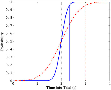
Figure 1. Standard normal cumulative distribution functions with the same mean (i.e., 2 s) but different coefficients of variation (CV, σ/μ). Solid curve illustrates the normal cdf for a CV of 0.1 and the dotted curve illustrates the normal cdf for a CV of 0.3. The probability of a random variable taking on a value shorter than the trial time, indicated by vertical solid and dotted lines, respectively, is 0.95. Note that this value is much lower for the simulated subject with smaller timing uncertainty (solid curve).
We now discuss temporal decision-making scenarios for which optimal decisions depend explicitly on the level of timing uncertainty. For these tasks, we formalize optimality as a function of the level of timing uncertainty and then compare the performance of humans and rodents to optimal performance given the observed level of timing uncertainty.
When to Switch from a Rich to a Poor Prospect
Using a task similar to that of Brunner et al., (1992; see also Balci et al., 2008), Balci et al. (2009) investigated the extent to which humans and mice behave normatively in incorporating estimates of endogenous timing uncertainty into temporal decisions made in the face of additional, exogenous uncertainty. In their experiment, subjects tried to anticipate at which of two locations a reward would appear. On a randomly scheduled fraction of the trials, it appeared with a short latency at one location; on the complementary fraction, it appeared after a longer latency at the other location. Switching prematurely on short trials or failing to switch in time on the long trials yielded either no reward, or yielded a penalty, depending on the payoff matrix. The exogenous uncertainty was experimentally manipulated by changing the probability of a given trial type (short or long). For humans, the payoff matrix was also manipulated by changing the magnitude of rewards and penalties associated with different consequences (e.g., switching early on a short trial). Mice received equal rewards and no penalty.
The optimal response policy in this “switch task” is to begin each trial assuming that the reward will occur at the short location, and when the short interval elapses with no reinforcement, to switch to the long location. The trial time at which the subject leaves the short option for the long one is called the “switch latency.” Switch latencies were normally distributed, to a close approximation. The mean of the best-fitting normal distribution was assumed to represent the subject’s target switch latency, and the coefficient of variation (CV = σ/μ) was taken to reflect endogenous timing uncertainty.
The expected gain (EG) for a given target switch latency is the sum of the relative values of the options. The relative value is the gain for a given option weighted by the probability of attaining it. In this case, it is the payoff matrix weighted by the probability of the corresponding consequences determined jointly by endogenous timing uncertainty and exogenous uncertainty (i.e., probability of a short trial). Equation 1 defines the EG for an estimate of target switch point  and endogenous timing uncertainty
where  is the subject’s temporal criterion for switching, TS and TL are the short and long referents, p(TS) is the probability of a short trial, and g denotes the payoff matrix [e.g., g(TS) reflects the payoff for a correct short trial and g(∼TS) reflects the loss for an incorrect short trial]. Φ is the normal cdf with mean
  and SD
  evaluated at TS or TL.
Figure 2 depicts the dependence of optimal switch latencies on the timing uncertainty for a given payoff matrix and on two exogenous probability conditions. For equally probable durations, the optimal switch latency (to, the t that maximizes the EG in Eq. 1) approaches the short target interval TS as the timing uncertainty ω increases, due to scalar timing noise. Different combinations of the probability of a short trial p(TS), and the payoff matrix g, result in different EG surfaces (gain for each combination of t and ω). Figures 2A,B depict the normalized EG surface for p(TS) = 0.5 and p(TS) = 0.9, respectively, with a penalty for early and late switches. Balci et al. (2009) compared the empirical target switch latencies  to optimal switch latencies
  for the estimated level of timing uncertainty
  by experimentally manipulated exogenous uncertainty p(TS), and the payoff matrix g. They found that both mice and humans performed nearly optimally in this task, achieving 99 and 98% of the maximum possible expected gain (MPEG), respectively. The average slopes of the orthogonal regression between empirical and optimal target switch latencies were 0.81 and 1.05 for human and mouse subjects, respectively (Figure 3A: Humans; B: Mice). These values were significantly different from 0 (both ps < 0.05) but not from 1 (both ps > 0.5). These results indicate that subjects tracked the optimal target switch latencies.
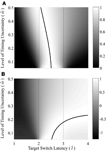
Figure 2. Expected gain surface (normalized by the maximum expected gain for different levels of timing uncertainty) as a function of target switch latency and the level of timing uncertainty  . Shades of gray indicate the percentage of normalized maximum expected gain for the corresponding parameter values,
  and
and  (A) is for equally probable short (2 s) and long (3 s) target intervals p(TS) = 0.5. The ridge of this surface (bold black curve) shows the optimal switch latencies for different levels of timing uncertainty. (B) is for a higher probability of the short target interval, p(TS) = 0.9. For both cases note the dependence of optimal target switch latencies on the level of timing uncertainty (y-axis). Also note the differences in optimal target switch latencies for two different exogenous uncertainty conditions.
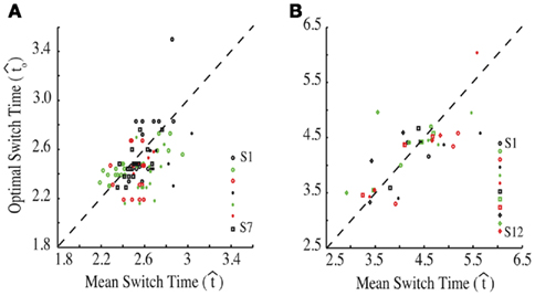
Figure 3. Empirical performance of human and mouse subjects as a function of optimal performance, calculated for the critical task parameters and subjects’ estimated level of endogenous timing uncertainty. Dashed line denotes the identity line. S: subject. Reprinted from Balci et al. (2009). (A) Humans; (B) Mice.
In line with reports reviewed earlier, these findings showed that humans and mice adapted performance to account for their endogenous timing uncertainty. It further demonstrated that subjects performed nearly optimally in adapting to exogenous uncertainty and to payoffs along with their endogenous uncertainty: i.e., they planned their timed responses such that they nearly maximized their expected earnings. This experiment thus lends strong support to the hypothesis that both humans and rodents can optimally assess temporal risk in certain contexts.
However, this work addresses only decisions about temporal intervals between a stimulus and a reward in a discrete-trial paradigm. Many natural tasks, on the other hand, are better characterized as free-response paradigms. Unlike discrete-trial tasks, these tasks impose tradeoffs between the speed and accuracy of decisions that are analogous to speed–accuracy tradeoffs in perceptual decision-making (see The Drift–Diffusion Model – An Optimal Model for Two-Choice Decisions). A prototypical timing task with this property is the differential reinforcement of low rates of responding (DRL) task. This task poses an interesting, naturalistic problem in which reward maximization depends on achieving the optimal level of patience, which is equivalent to finding the optimal tradeoff between two time-dependent quantities (as we now describe). In the following section, we will use reward rate (RR) in place of “EG” since we will evaluate the performance in free-response rather than discrete-trial protocols.
Optimal Tradeoff between Two Time-Dependent Quantities (New Experiment)
In the DRL task, subjects are taught to space each successive response so that it occurs after a fixed minimum interval (or “withhold duration”) since the last response. Each response immediately starts a new trial and only those responses emitted after the minimum withhold duration are rewarded. For instance, in a DRL 10 s schedule, subjects are reinforced for responding after at least 10 s following the previous response. If they respond sooner, then the trial timer restarts with no reward. Reward maximization in this simple task depends on the optimal tradeoff between two time-dependent quantities with opposing effects on the rate of reward: the probability of reward, p(R), and the average IRT. The reward probability increases as IRTs increase (serving to increase the RR), but with sufficiently long IRTs, the mean inter-reward interval increases as well. The RR is the probability of reward divided by the average time between responses (see Eq. 2):
Importantly, the optimal tradeoff between p(R) and IRT that maximizes RR depends on the subject’s endogenous timing uncertainty (see also Wearden, 1990). Equation 3 defines the RR in the DRL task assuming inverse Gaussian (Wald) distributed IRTs. This assumption accurately describes our DRL data, and it is consistent with a recently developed random walk model of interval timing (Rivest and Bengio, 2011; Simen et al., 2011). In this model, a noisy representation of time rises at a constant rate (on average) as time elapses. Responses are emitted when this increasing quantity crosses a single, strictly positive threshold (this model is described in more detail in the discussion). Our inverse Gaussian assumption also accurately describes other human and animal datasets from paradigms in which subjects emit a single response or a target interval can be estimated (see Simen et al., 2011). For the DRL procedure, the expected RR for a given, normalized target IRT  and a given level of timing uncertainty
  is:
is:

Here, T is the DRL schedule,  is the schedule-normalized mean IRT (i.e., the average target withhold duration divided by the DRL schedule), and
  is the Wald distribution’s shape parameter, which captures the noisiness of the underlying random walk (the Wald cumulative distribution function – waldcdf in Eq. 3 – is defined in the Appendix). The timing uncertainty equals the coefficient of variation, or SD divided by the mean, of this IRT distribution.
Figure 4 shows the normalized EG surface for the DRL task as defined by Eq. 3. The ridge of the surface (dark solid line) denotes the optimal IRTs as a function of timing uncertainty  . As the coefficient of variation increases, the optimal IRT diverges from the DRL schedule in a negatively accelerating fashion.
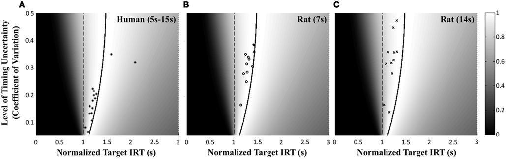
Figure 4. Normalized expected reward rate surface as a function of the normalized target IRT and the level of timing uncertainty. Shades of gray denote the proportion of normalized MPEG, which decreases from light to dark. The solid black curve is the ridge of the normalized expected reward rate surface and denotes the optimal IRT for different levels of timing uncertainty. The dashed vertical black line shows the normalized DRL schedule (in actuality ranging from 5 to 15 s). Each symbol corresponds to the performance of a single rat or human subject in the novel experiment. (A) (Asterisks) shows the human data (DRL 5–15 s), (B) (circles) shows the rat data (DRL 7 s) and (C) (crosses) shows the rat data (DRL 14 s). Data points were clustered near and to the left of the ridge of the expected reward rate surface.
Methods
To assess the optimality of rat and human DRL performance, we tested rats in a new experiment for 42 sessions with 7, 14, 28, and 56 s DRL schedules1 (∼12 rats per group), and humans in single session experiments with DRL schedules that ranged between 5 and 15 s (varied across participants). Methodological details of these experiments are presented in the Appendix. Rats exhibited two types of responses: timed and untimed. This created a mixture distribution for the IRTs that was best fit by an exponential-Wald mixture distribution. The IRTs that were best fit by the exponential component were considered to be untimed responses, which occurred relatively quickly after the previous response. The IRTs that were best fit by the Wald component were considered to be timed responses.
Results
Human performance. Figure 4A depicts the performance of humans (asterisks). It suggests that humans tracked the modulation of optimal IRTs as a function of temporal uncertainty. Statistical analyses corroborated these observations. The median performance of humans provided 98% [interquartile interval (IQI) 4%] of the MPEG. Similar estimates of nearly maximal EG were obtained when we used an independent estimate of endogenous timing uncertainty from a temporal reproduction task with parametric feedback on each trial (see Appendix for details). Optimal IRTs were significant predictors of the empirical IRTs, R2 = 0.56, F(1,13) = 16.29, p < 0.01. When one outlier was excluded from the dataset (using 2 SD as the exclusion criterion), this relation became even stronger and more reliable, R2 = 0.71, F(1,12) = 29.45, p < 0.001. During debriefing this outlier participant reported that s/he was not engaged in the task. Humans’ earnings were significantly larger than what they would have earned if they had aimed at the schedule, t(14) = 11.06, p < 0.0001, and their empirical IRTs were significantly longer than the minimum withhold duration, t(14) = 3.96, p < 0.01. When data were fit with an exponential–Gaussian mixture distribution instead, the median earnings were 99% of the MPEG.
Rat performance. Median performance of rats for 7 and 14 s DRL schedules were 98% (IQI 3%) and 96% (IQI 5%) of the MPEG. Figures 4B,C show that rats’ average withhold durations tracked the optimal duration. Corroborating this observation, optimal IRTs were significant predictors of empirical IRTs for both 7 and 14 s schedules, R2 = 0.60, F(1,10) = 14.68, p < 0.01 and R2 = 0.38, F(1,9) = 5.60, p < 0.05, respectively. The earnings of rats were significantly larger than they would have been if they had aimed for the DRL schedule itself for 7 s [t(11) = 18.97, p < 0.0001], and 14 s [t(10) = 6.84, p < 0.0001]. Empirical IRTs were significantly longer than the minimum withhold duration for 7 s [t(11) = 11.42, p < 0.0001], and 14 s [t(10) = 7.30, p < 0.0001]. When data were fit with an exponential–Gaussian mixture distribution instead, median proportions of the MPEG were 99% for both schedules.
In a theoretical work, Wearden (1990) conducted essentially the same analysis as ours to characterize the optimal target IRTs in the DRL task. He showed that linear “overestimation” of the DRL was the optimal strategy, and that the degree of overestimation depended on the level of timing uncertainty. His reanalysis of a pigeon dataset (Zeiler, 1985) from a DRL-like task revealed nearly optimal “overestimation” of the scheduled reinforcement availability time. Wearden’s reanalysis of human DRL data from Zeiler et al. (1987), with target intervals ranging from 0.5 to 32 s, also revealed very nearly optimal performance. Our secondary analyses of two independent, published datasets from rats corroborated our and Wearden’s observations from rats, pigeons, and humans. We compared the performance of control group rats in Sanabria and Killeen(2008 – 5 s DRL), and Orduña et al., (2009 – 10 s DRL) to the optimal performance computed for their estimated levels of timing uncertainty. Rats in these experiments achieved 93, and 94% of the MPEG for 5 and 10 s schedules, respectively, under an exponential-Wald fit. These values reached 96% for both datasets, when exponential–Gaussian mixture distributions were fit to the data instead.
Other examples can be found in the literature in which IRT distributions peak long after the DRL schedule at least for schedules up to 36 s. These data qualitatively corroborate our observations [e.g., Fowler et al., 2009 (Figure 2A); Stephens and Cole, 1996 (Figure 4A), Cheng et al., 2008, (Figures 5 and 6), Sukhotina et al., 2008 (Table 1 and Figure 3)]. With longer DRL schedules (e.g., DRL 72 s), on the other hand, subjects perform pronouncedly sub-optimally [e.g., Balcells-Olivero et al., 1998 (Figure 1), Fowler et al., 2009 (Figure 2B), Paterson et al., 2010 (Figures 1–4)]. In line with our observations with 28 and 56 s DRL schedules, the sub-optimal performance in longer schedules might simply be due to the need for longer training. Wearden (1990) alternatively argued that the “underestimation” of the DRL schedules might be due to a satisficing strategy to obtain a certain satisfactory rate of reinforcement, an adaptive response bias the extent of which also depends on the level of endogenous timing uncertainty (Wearden, 1990, Figure 4). Overall, in line with our findings from the discrete-trial switch task, human and rat performance in the free-response DRL task suggests that these species can assess temporal risk optimally when timing uncertainty is a determinant of the optimal tradeoff between waiting and responding.
In the DRL task, subjects are not rewarded (thereby suffering an opportunity cost) for responding prior to the minimum response–withholding duration. On the other hand, being late is also commonly “penalized” in nature, as in the case of losing a precious resource to a competitor by virtue of not claiming it early enough. In the next section, we describe a task with this characteristic, in which reward maximization requires avoiding late responses, and we re-evaluate human performance data from Simen et al. (2011) within the framework of optimality.
Beat-the-Clock Task
In the beat-the-clock (BTC) task (Simen et al., 2011), participants are asked to press a key just before a target interval elapses, but not afterward. The reward for responding grows exponentially in time, increasing from approximately 0 cents immediately after the cue appears to a maximum of 25 cents at the target interval. Thus responding as close to the target interval as possible is adaptive. Failing to respond prior to the target interval is not rewarded (imposing an opportunity cost). Response times collected in the BTC task were best fit by a Gaussian distribution, with the mean reflecting the target response time and the CV reflecting endogenous timing uncertainty. Equation 4 defines the EG for a given target response time  timing uncertainty
  and schedule T.

where t is a possible response time,  is the target response time, p is the probability of responding at t given the subject’s mean
  and coefficient of variation
  and g is the exponentially increasing reward function that drops to zero after the deadline. The optimal aim point to is the one that maximizes EG for a given level of timing uncertainty
  We performed a secondary data analysis on this dataset, originally presented in Simen et al. (2011). Figure 5 depicts the dependence of optimal aim points on psychologically plausible levels of timing uncertainty and shows that human participants tracked the optimal target times.
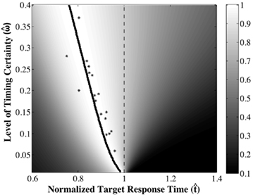
Figure 5. Normalized expected gain surface as a function of normalized aim point and level of timing uncertainty. Shades of gray denote the proportion of normalized MPEG, which decreases from light to dark. The black curve is the ridge of the expected gain surface and denotes the optimal aim points for psychologically plausible levels of endogenous timing uncertainty. Each point (asterisk) corresponds to the performance of a single subject and points are clustered around the curve of the optimal aim points. Figure is redrawn based on the data presented in Simen et al. (2011).
Consistent with Figure 5, optimal target times were significant predictors of empirical target times [R2 = 0.76, F(1,15) = 47.67, p < 0.0001). Participants earned 99% median (IQI 3%) of the MPEG for their level of timing uncertainty. The proportion of earnings was 99% median (IQI 2%) of the MPEG when the timed responses were assumed to be Wald distributed, instead. As in the switch and DRL tasks, these results suggest a nearly optimal human capacity for taking endogenous timing uncertainty into account when planning timed responses – in this case, in scenarios in which late responding is maladaptive.
In three different temporal decision-making tasks that impose different time constraints on the problem of reward maximization, we have demonstrated that optimal performance depends on endogenous timing uncertainty. We have further demonstrated that humans, rats, and mice incorporate their endogenous timing uncertainty nearly optimally in their temporal risk assessment, at least for supra-second target durations.
Optimality in the Sub-Second Range
The characterization of temporal risk assessment in the switch, DRL, and BTC tasks pertains exclusively to decisions about supra-second intervals. There is, however, substantial evidence that different neural circuits might underlie supra-second and sub-second intervals (e.g., Breukelaar and Dalrymple-Alford, 1999; Lewis and Miall, 2003). Thus, there is reason to believe that optimality of temporal risk assessment might be exclusive to supra-second interval timing. Using a simple temporal reproduction task with humans, however, Jazayeri and Shadlen (2010) showed that optimal temporal risk assessment also applies to sub-second target durations.
In their task, participants were asked to reproduce time intervals that were sampled from different underlying distributions (including sub-second intervals). When reproductions fell within a temporal window of the target interval, participants received positive feedback. The resulting reproductions of target intervals were observed to regress to the mean of the encountered intervals, and thus the reproduction of the same interval could change depending on the underlying distribution of intervals experienced. Importantly, Jazayeri and Shadlen (2010) demonstrated that a reward-maximizing model that took account of the statistics of the target interval distribution and incorporated knowledge of scale-invariant endogenous timing uncertainty accounted for the performance of the participants. Their findings demonstrate that humans take normative account of endogenous timing uncertainty to maximize reward, even in the case of sub-second target durations. Temporal decision-making with sub-second target intervals is more common in simple motor planning tasks, which we discuss next.
Optimal Motor Timing
Hudson et al. (2008) reported an experiment in which human participants were asked to touch a computer screen at a particular time (e.g., 650 ms) to earn monetary reward. A small time window around this target interval served as the reward region (e.g., 650 ± 50 ms). There was also a penalty region, which imposed monetary costs. Lastly, there was a region in which neither reward or penalty occurred. The temporal position of the penalty region was manipulated. Sometimes it perfectly straddled the reward region (and anything outside the reward region was penalized). Sometimes it was adjacent to the reward region on one side but not the other (thus aiming toward the other side was a good strategy). The participant’s task was to maximize the monetary reward during the course of the experiment.
There were two sources of variance: (1) the participants’ own timing uncertainty (ω) and (2) experimentally added exogenous noise (α) that was applied to every temporal aim point (drawn from a Gaussian with μ = 0 and σ = 25 ms). Empirical data suggested that participants incorporated both endogenous and exogenous temporal uncertainties (ω and α) as they aimed at a time that very nearly compensated for both the timing uncertainty and the payoff matrix (i.e., the temporal positions of the reward and penalty regions). Thus, consistent with earlier reports, these findings showed that humans can take nearly normative account of their endogenous timing uncertainty and that they can also learn to take account of experimentally introduced temporal noise in planning their movement times. Analogous nearly optimal timing of single isolated movements was also reported in other studies (e.g., Battaglia and Schrater, 2007; Dean et al., 2007).
Further work (Wu et al., 2009), however, discovered a bound for optimal performance in these tasks and showed that optimality of timed motor planning does not hold when subjects are asked to allocate time across two options to complete a sequence of movements under stringent time pressure (i.e., 400 ms). Specifically, they observed that subjects spent more time than optimal on the first target, even when the payoff for the second target was five times larger. Based on this finding, Wu et al. (2009) claimed that the optimality of motor timing is restricted to isolated, single movements, and fails in the context of a sequence of movements. One important feature of their task that should be considered, however, is the very stringent response deadline imposed on the completion of the movement sequence (although subjects could take as much time as they wanted before initiating the trial). These findings overall suggest that except in the case of a sequence of movements made under a strict response deadline, humans exercise optimal motor timing with sub-second target intervals.
In the last two sections, we described decision-making scenarios that were explicitly temporal in nature, both with sub-second and supra-second target durations. In these tasks, subjects made explicit judgments about time intervals and exhibited optimal temporal risk assessment. The adaptive role of interval timing is however not at all limited to explicitly temporal decision-making. It also plays a crucial but understudied role in reward maximization in perceptual decision-making. In free-response paradigms for instance, timing uncertainty interacts with two-choice performance because reward maximization requires subjects to keep track of RRs and thus inter-reward times. In the case of time-pressured decisions (i.e., with response deadlines), interval timing is even more directly instrumental for reward maximization, since optimality then requires taking account of the deadline, as well as uncertainty in its representation. In the next section, we discuss the role of interval timing in perceptual two-choice decision-making tasks.
Interval Timing and Reward Maximization in Non-Temporal Decision-Making
The likely connection between RR estimation and time estimation suggests that endogenous timing uncertainty should translate into uncertainty about RRs. As we describe below, within the framework of optimality, this dependence generates a prediction that a decision-maker with higher timing uncertainty will respond more slowly than optimal (favoring accuracy over RR) in free-response two-choice tasks (Bogacz et al., 2006). Under this hypothesis, Bogacz et al. (2006) and Balci et al. (2011) argued that such “sub-optimally” conservative responding in these paradigms might in fact reflect an adaptive bias in decision threshold setting in response to endogenous timing uncertainty. Our analysis and discussion of optimal temporal risk assessment in these tasks will heavily rely on the drift–diffusion model (DDM) of two-choice decisions, which we describe next.
The Drift–Diffusion Model – an Optimal Model for Two-Choice Decisions
The sequential probability ratio test (SPRT; Barnard, 1946; Wald, 1947) is an optimal statistical procedure for two-alternative hypothesis testing in stationary environments that provide an unlimited number of sequential data samples. The SPRT minimizes the number of samples for any given level of accuracy, and maximizes accuracy for any given number of samples (Wald and Wolfowitz, 1948). In an SPRT-based model of choice reaction time in two-choice tasks, Stone (1960) proposed that decision-makers computed the likelihood ratio of the two hypotheses when sampling a noisy signal, equating the total sample count with the decision time. In the DDM this discrete sequence of samples is generalized to a continuous stream, in which the time between samples is infinitesimal (Ratcliff, 1978; Ratcliff and Rouder, 1998).
The DDM assumes that the difference between the evidence supporting the two hypotheses is the decision variable, that this variable is integrated over time, and that when the integrated evidence crosses one of two decision thresholds – one (+z) above and one (−z) below the prior belief state – the corresponding decision is made. The first crossing of a threshold is identified as the decision time. The DDM in its most simplified form, is given by a first order stochastic differential equation in which x denotes the difference between the evidence supporting the two different alternatives at any given time t; it can be interpreted as the current value of the log-likelihood ratio:

Here, Adt represents the average increase in x during the tiny interval dt, and σdW represents white noise, Gaussian distributed with mean 0 and variance σ2dt (see Ratcliff and McKoon, 2008 for a detailed description of the DDM).
In the DDM, the clarity of the signal is represented by the drift A (the signal-to-noise ratio is A/σ). Speed–accuracy tradeoffs arise in the DDM because of the threshold parameter z: Due to noise, lower thresholds lead to faster but less accurate decisions and vice versa. The pure form of the DDM in Eq. 5 (e.g., Ratcliff, 1978) often provides reasonably good fits to behavioral data, and benefits from extremely simple, analytically tractable predictions regarding RR maximization (Bogacz et al., 2006). Versions of the DDM with additional parameters (e.g., Ratcliff and Rouder, 1998) are needed for fitting a broader range of data, especially data with unequal mean RTs for errors and correct responses.
Optimal Two-Choice Decision-Making and Interval Timing
The pure DDM (i.e., a model without the additional variability parameters used in the model of Ratcliff and Rouder, 1998) prescribes a parameter-free optimal performance curve that relates decision time to error rate (Bogacz et al., 2006). Optimal performance, however, requires decision thresholds that are a function of the response-to-stimulus interval (RSI). Better estimation of the RSI by participants with more precise timing abilities may therefore result in better decision-making performance. Deviations from optimal performance may thus derive from timing uncertainty. The shape of the function relating the expected RR to the decision threshold in the DDM suggests why this may be the case. Specifically, this function is an asymmetric hill, whose single peak defines the optimal threshold. For a given level of deviation from the optimal threshold, setting the threshold too high earns a higher expected RR than setting it too low by the same amount [Balci et al., 2011 (Figures 7 and 10), Bogacz et al., 2006 (Figure 15)]. Thus, if decision-makers are to minimize loss in RR due to endogenous timing uncertainty in RR estimates, they should err toward overestimating instead of underestimating the optimal threshold. The behavioral manifestation of overestimating a threshold is longer response times coupled with greater accuracy (which in model fits appears to suggest a suboptimal, “conservative,” emphasis on accuracy over speed, and thus RR).
In a single session of two-alternative forced choice tasks, human participants have indeed been shown to set their decision thresholds higher than the optimal decision threshold (Bogacz et al., 2010). Balci et al. (2011) replicated this finding (but also showed that this deviation decreased nearly to zero with sufficient practice) and observed that deviations from optimality during early training could be accounted for by participants’ timing uncertainty (assessed independently). Balci et al. (2011) quantified deviation from optimality in two different ways: (1) deviations between optimal and observed RTs; and (2) deviations between optimal and fitted thresholds. For both measures, Balci et al. (2011) reported that the regression of deviations from optimality on CVs revealed a significant relationship F(1,15) = 12.1, p < 0.01 (R2 = 0.45) and F(1,14) = 22.57, p < 0.001 (R2 = 0.62; excluding one outlier based on a 2 SD rule), respectively (see Figure 6). They also reported that this relationship held even after first accounting for suboptimal performance by another model that included a parameter representing a self-imposed penalty for errors (Maddox and Bohil, 1998; Bogacz et al., 2006).
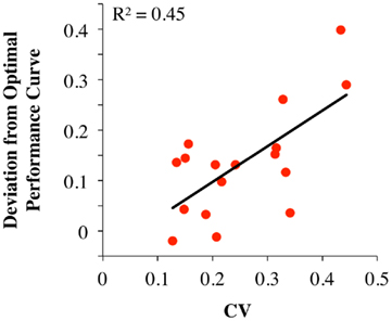
Figure 6. Deviation from the optimal performance curve of the pure DDM as a function of CV redrawn based on the data presented in Balci et al. (2011). Solid line is the linear regression line fit to the data.
Zacksenhouse et al. (2010) recently analyzed the data presented in Bogacz et al. (2010) using a decision strategy that maximized the minimal RR achievable for a given level of timing uncertainty. This decision strategy fit the Bogacz et al. (2010) dataset better than an optimally parameterized DDM, and better than the alternative models that contained an assumed penalty for errors. Conservative decision thresholds can therefore be viewed as an intrinsic, adaptive bias in response to endogenous timing uncertainty, a dynamic that underlies nearly optimal performance in the switch, BTC, and DRL tasks. These findings suggest the importance of timing uncertainty in shaping behavior and determining how much reward is earned even in non-temporal decision-making.
Two-Choice Decision-Making Under Time Pressure
Interval timing plays a more direct role in two-choice decisions when a response deadline sets an upper bound for rewarding responses and/or for viewing time. Frazier and Yu (2008) showed that optimal performance in these scenarios requires subjects to start collapsing decision thresholds so that by the time the deadline is reached, the decision threshold converges on the starting point of the accumulation process (see also Rapoport and Burkheimer, 1971; Latham et al., 2007; Rao, 2010). This strategy ensures that a decision is made prior to the response deadline while maximizing accuracy for a given response time. According to this model, for a given level of timing uncertainty, subjects should start collapsing decision thresholds earlier for shorter response deadlines. Conversely, for a given response deadline, subjects with higher timing uncertainty should start collapsing decision thresholds earlier compared to subjects with lower timing uncertainty. We are currently testing these two specific predictions with human subjects. Preliminary results do not fully support the notion of optimal, within-trial modulation of response thresholds. Nevertheless, they do suggest some amount of threshold modulation within and across trials in response to changing deadlines. They further suggest a relation in the expected direction between the level of subjects’ timing uncertainty and the degree of accuracy reduction in their conditional accuracy (or micro speed–accuracy tradeoff) curves in response deadline conditions (i.e., accuracy levels in each of a set of binned RTs, which should be flat for the pure DDM with a fixed threshold, but which must decrease for RT bins near the deadline if thresholds collapse).
Discussion
Time is a defining feature of behavior. By incorporating the well-characterized psychophysics of interval timing into the study of reward maximization, we have demonstrated that temporal intervals and uncertainty in their representation are critical factors in both temporal and non-temporal decisions. The findings we reviewed show that humans and animals come close to maximizing their earnings in simple timing and decision-making tasks, which suggests that they can normatively compensate for their endogenous timing uncertainty in their decision-making. Subjects nearly maximized the reward earned in scenarios that spanned sub-second and supra-second target durations, in the presence and absence of speed–accuracy tradeoffs (i.e., free-response vs. fixed viewing time), and explicitly temporal and perceptual decisions.
These findings contrast with the assertions of classical decision-making research that has repeatedly shown that humans are irrational decision-makers about probabilistic prospects (e.g., Kahneman and Tversky, 1979). Here, we have shown that when uncertainty is endogenous and specifically temporal in nature, humans in fact make nearly optimal decisions. Supporting this view, a series of experiments on motor planning have also shown that humans decide (plan their motor end-points) optimally when confronted with other ubiquitous sources of endogenous uncertainty, such as motor noise (e.g., Trommershäuser et al., 2008). These results suggest that when the origin of uncertainty is endogenous, as in interval timing or motor planning, the resulting uncertainty is accounted for by mechanisms that organize and adapt behavior optimally in response to environmental statistics. We note, however, that these findings do not necessarily indicate that endogenous uncertainty is explicitly represented via a domain-general, metacognitive ability. They simply show that humans and other animals can make decisions that are adapted to endogenous timing uncertainty in a way that tends to maximize rewards. Depending on the task representation (avoiding being early or late), the level of timing uncertainty can be implicitly translated into a response bias signal that in turn partially determines the temporal characteristics of behavior. In fact, the task representation might simply determine the direction, whereas the timing uncertainty might determine the magnitude, of the response bias.
An important observation with humans is that reward maximization in perceptual decision-making (i.e., dot motion discrimination) requires extensive training (e.g., Simen et al., 2009; Balci et al., 2011), whereas optimal performance in temporal decision-making appears within a single session: i.e., in the switch task (Balci et al., 2009), DRL (current experiment), and BTC (Simen et al., 2011). This difference is possibly due to the relatively extensive exposure of humans to temporal intervals compared to the specific visual stimuli (e.g., dot motion patterns) typically used in perceptual decision-making tasks. Time, after all, is a fundamental quantity that factors critically into the outcome of almost all human and animal behavior. The ubiquity of time experience may have allowed animals to establish a veridical, scale-invariant model of their endogenous timing uncertainty, which can be used normatively in decision-making. Estimating the signal-to-noise ratios of novel stimuli (e.g., dot motion stimuli), on the other hand, requires extensive new training, which is likely the primary factor in the delayed achievement of optimal performance in perceptual decision-making. Timing might therefore appear to be a special case in which optimal decisions are made in single session experiments simply due to the degree of previous experience. Consistent with this interpretation, when timing uncertainty also has an exogenous source, human participants require some additional experience before exhibiting optimal performance (Hudson et al., 2008).
In addition to addressing the optimality of temporal risk assessment, a reward maximization framework also offers a novel, principled resolution to a psychophysical controversy in the domain of interval timing: namely the location of the point of subjective equality (PSE) between different durations. The PSE is the time interval that is subjectively equidistant to two other intervals, which subjects are equally likely to categorize as short or long. The PSE for animals is often found to be close to the geometric mean of the referents (e.g., Church and Deluty, 1977) but closer to the arithmetic mean for humans (e.g., Balci and Gallistel, 2006). This inconsistency has been a source of theoretical controversy because of its implications regarding the subjective time scale – i.e., whether it is logarithmic or linear (Montemayor and Balci, 2007; Yi, 2009). The optimality-based account of temporal discrimination (switch or bisection) performance offers a principled account of the location(s) of the PSE; it quantitatively predicts this difference based on cross-species differences in the level of endogenous timing uncertainty on a linear subjective time scale.
The switch task is essentially a free-operant variant of the temporal bisection task, in which subjects can emit responses throughout the trial rather than just a single, terminal choice after an experimenter-determined probe interval elapses. In fact, in temporal bisection trials, animals move from the short to the long response option as the elapsed time approaches and exceeds the PSE (Machado and Keen, 2003). This suggests that despite the retrospective nature of the temporal bisection task, animals make real-time judgments about the elapsing interval in this task, just as in the case of the switch task. Balci and Gallistel (2006) further showed that in temporal bisection tasks, human participants set a single criterion between the referents and judge intervals as short or long relative to that criterion (see also Allan, 2002; Penney et al., 2008).
Based on the parallels between decision strategies employed in both temporal discrimination tasks, the expected reward function of the switch task also applies to the temporal bisection task. Accordingly, when Figure 2A is evaluated for the temporal bisection task, where the short and long target intervals refer to the short and long reference durations, it predicts that PSEs are closer to the geometric mean for higher endogenous timing uncertainty (as in animals) and closer to the arithmetic mean for lower endogenous timing uncertainty (as in humans). This account, based on the same principles, also predicts the effect of task difficulty (short/long ratio) on the location of the PSE in humans (Wearden and Ferrara, 1996): more difficult task conditions mimic higher timing uncertainty and easier task conditions mimic lower, and the PSE moves across conditions accordingly.
Finally, for the rat DRL dataset, we only considered what are referred to as “timed responses” for our optimality analysis (see also Wearden, 1990). Wearden (1990) showed that untimed short responses (responses occurring almost immediately after the preceding response) did not exert much cost on the reward earned in the DRL task. For instance, 75% of untimed mostly short responses (uniformly distributed between 0.25 and 0.75 s) resulted in 92% of the reward that could be obtained without any untimed short responses for a DRL 20 s schedule, mean IRT of 20 s, and CV of 0.3. We further argue that particularly given their low cost regarding reward earned, untimed short responses could in fact constitute an optimal strategy in the long run for non-stationary environments. For instance, these responses would enable subjects to detect a shift to a richer schedule (DRL20 → DRL10 s) and thus adjust responding accordingly. On the other hand, the detection of this change would be more difficult and/or delayed for a subject who exclusively exploits the DRL schedule (i.e., emitting only timed responses).
Despite our claim about the ability of humans and non-human animals to account for their endogenous timing uncertainty, we have not proposed a mechanistic account of this ability. What are the possible mechanisms by which organisms infer and represent their timing uncertainty? We assume that this ability relies on keeping track of the discrepancies between the time of maximal expectancy of an event and the actual time of its occurrence over many instances. The stochastic ramp and trigger (SRT) model of Simen et al. (2011) allows keeping track of such experiential discrepancies. The SRT model approximates a drift–diffusion process with a single, fixed threshold, and a noise coefficient proportional to the square root of the drift (see also Rivest and Bengio, 2011). This model, which contains the Behavioral Theory of Timing of Killeen and Fetterman (1988) as a special case (where accumulation is effectively a pulse counting process), exploits the same mechanism used to account for response times in decision-making. In the simplest terms, the model times an interval by accumulating a quantity at a constant rate until it crosses a threshold, call it z. This accumulation is perturbed by the addition of normally distributed random noise with mean 0. Time intervals of duration T are timed by setting the accumulation rate (the “drift”) equal to the threshold divided by T, and simple learning rules can tune the drift to the right value after a single exposure to a new duration. The resulting threshold crossing times exhibit scalar invariance and predict response time distributions that account for human and animal empirical data.
Importantly, as in models of decision-making (e.g., Simen et al., 2006), adjustments can be made in the intended time of responding relative to T by setting a response threshold that is either higher or lower than the timing threshold. Optimality requires that it be higher for the DRL task, and lower for the BTC task. Although this threshold-adjustment approach to optimizing timed performance appears to be novel in the timing literature, it is standard fare in the literature on perceptual decision-making. Thus, both the underlying model (the drift–diffusion process) and the techniques for adapting its speed–accuracy tradeoffs (via threshold-adjustment) emerge as potentially common computational principles in two distinct psychological domains.
The SRT model allows keeping track of discrepancies from veridical times. When ramping activity hits the threshold prior to the occurrence of the event (early clock), the organism can time the interval between the threshold crossing and the event. Likewise, when ramping activity fails to hit the threshold at the time of the event (late clock), the organism can now time the interval between the event and projected threshold crossing. When these values are divided by the target interval (threshold/drift), it indicates the scale-invariant measure of endogenous timing uncertainty. Simen et al. (2011) in fact used these values to adjust the clock speed to time veridical intervals in their model (see also Rivest and Bengio, 2011, where the same learning rules were proposed). The same mechanism can be conveniently used to keep track of timing noise through experience.
How this function might be embedded in the neural circuitry (i.e., corticostriatal loops) that have been implicated in interval timing is an important question that deserves special attention. In parallel to the striatal beat frequency model (Matell and Meck, 2004), different roles can be assigned to different brain regions within the SRT framework. For instance, the clock role can be assigned to the cortex and the effective role of decision threshold to the striatum. Within this scheme, it is possible that the reinforcement contingent dopamine activity serves as a teaching signal, which, via long-term synaptic plasticity (i.e., LTP and LTD), changes the excitability of the striatal medium-spiny neurons that are innervated by cortical glutamatergic and nigral dopaminergic input. This activity might effectively set the decision thresholds in the direction and magnitude that maximizes the RR. In cases where the reward function depends on endogenous timing uncertainty, dopamine activity would thus inherently serve as a signal of the interaction between endogenous timing uncertainty and task structure. In tasks like the DRL and BTC, brain regions involved in inhibitory control (e.g., orbitofrontal cortex) would also be assumed to factor into this process. This framework however suffers a critical problem, namely: “If the striatal neurons are ‘trained’ to respond specifically at intervals that maximize the reward (which are systematically shorter and longer than the critical interval), how do they represent the veridical critical temporal intervals?” This question suggests that the adaptive response bias signal should perhaps be assigned to an independent process controlled by an independent structure such as the orbitofrontal cortex. This scheme allows that task representation to be coded independently from the critical task parameter values.
There are two interesting issues, which should motivate and guide future research seeking a more comprehensive understanding of temporal risk assessment ability. One of these questions regards the correspondence between the temporal risk assessment performance of participants across multiple tasks. Considerable overlap between performances would constitute strong evidence for the assertion that the ability to account for timing uncertainty is an inherent (i.e., not entirely task-dependent) property of organisms. The second question regards the possible relation between decision-making performance under endogenous uncertainty (e.g., timing uncertainty) and exogenous uncertainty (e.g., discrete probability of reward delivery). Balci et al. (2009) observed close to optimal performance in a task that involved both kinds of uncertainties. However, it would be informative to test the same subjects in independent tasks in which the reward function depends exclusively on either endogenous or exogenous uncertainty in a given task.
In this paper, we have presented both published and novel datasets that support the claim that humans and other animals can take approximately normative account of their endogenous timing uncertainty in a variety of timing and decision-making tasks. This notion contrasts with the now-traditional view of humans as irrational decision-makers under uncertainty, a difference that may be driven by differences in the origin of the uncertainty (i.e., endogenous vs. exogenous uncertainty) and by the ways in which estimates of this uncertainty are acquired (i.e., by experience or by explicit description). Or it may be that timing is simply so critical for reward-maximizing behavior that the resulting selective pressure on animals’ timing abilities dominates the costs of maintaining those abilities.
Conflict of Interest Statement
The authors declare that the research was conducted in the absence of any commercial or financial relationships that could be construed as a potential conflict of interest.
Acknowledgments
The authors would like to thank Russell Church, Federico Sanabria, Peter Killeen, Vladimir Orduna, Lourdes Valencia-Torres, and Arturo Bouzas for making their data available to us. This work was supported by an FP7 Marie Curie PIRG08-GA-2010-277015 to FB, the National Institute of Mental Health (P50 MH062196, Cognitive and Neural Mechanisms of Conflict and Control, Silvio M. Conte Center), the Air Force Research Laboratory (FA9550-07-1-0537), and the European project COST ISCH Action TD0904, TIMELY.
Footnote
- ^Rat performance in DRL 28 and 56 s schedules did not reach steady state performance, and thus was not included in the analysis.
References
Balcells-Olivero, M., Cousins, M. S., and Seiden, L. S. (1998). Holtzman and Harlan Sprague–Dawley rats: differences in DRL 72-sec performance and 8-hydroxy-di-propylaminotetralin-induced hypothermia. J. Pharmacol. Exp. Ther. 286, 742–752.
Balci, F., Freestone, D., and Gallistel, C. R. (2009). Risk assessment in man and mouse. Proc. Natl. Acad. Sci. U.S.A. 106, 2459–2463.
Balci, F., and Gallistel, C. R. (2006). Cross-domain transfer of quantitative discriminations: Is it all a matter of proportion? Psychon. Bull. Rev. 13, 636–642.
Balci, F., Papachristos, E. B., Gallistel, C. R., Brunner, D., Gibson, J., and Shumyatsky, G. P. (2008). Interval timing in the genetically modified mouse: a simple paradigm. Genes Brain Behav. 7, 373–384.
Balci, F., Simen, P., Niyogi, R., Saxe, A., Hughes, J., Holmes, P., and Cohen, J. D. (2011). Acquisition of decision-making criteria: reward rate ultimately beats accuracy. Atten. Percept. Psychophys. 73, 640–657.
Battaglia, P. W., and Schrater, P. R. (2007). Humans trade off viewing time and movement duration to improve visuomotor accuracy in a fast reaching task. J. Neurosci. 27, 6984–6994.
Blough, D. S. (1967). Stimulus generalization as a signal detection in pigeons. Science 158, 940–941.
Bogacz, R., Hu, P. T., Holmes, P., and Cohen, J. D. (2010). Do humans produce the speed accuracy tradeoff that maximizes reward rate? Q. J. Exp. Psychol. 63, 863–891.
Bogacz, R., Shea-Brown, E., Moehlis, J., Holmes, P., and Cohen, J. D. (2006). The physics of optimal decision making: a formal analysis of models of performance in two-alternative forced choice tasks. Psychol. Rev. 113, 700–765.
Breukelaar, J. W., and Dalrymple-Alford, J. C. (1999). Effects of lesions to the cerebellar vermis and hemispheres on timing and counting in rats. Behav. Neurosci. 113, 78–90.
Brunner, D., Kacelnik, A., and Gibbon, J. (1992). Optimal foraging and timing processes in the starling, Sturnus vulgaris: effect of inter-capture interval. Anim. Behav. 44, 597–613.
Catania, A. C. (1970). “Reinforcement schedules and psychophysical judgments: a study of some temporal properties of behavior,” in The Theory of Reinforcement Schedules, ed. W. N. Schoenfeld (New York: Appleton-Century-Crofts), 1–42.
Cheng, R.-K., MacDonald, C. J., Williams, C. L., and Meck, W. H. (2008). Prenatal choline supplementation alters the timing, emotion, and memory performance (TEMP) of adult male and female rats as indexed by differential reinforcement of low-rate schedule behavior. Learn. Mem. 15, 153–162.
Church, R. M., and Deluty, M. Z. (1977). Bisection of temporal intervals. J. Exp. Psychol. Anim. Behav. Process. 3, 216–228.
Church, R. M., Lacourse, D. M., and Crystal, J. D. (1998). Temporal search as a function of the variability of interfood intervals. J. Exp. Psychol. Anim. Behav. Process. 24, 291–315.
Church, R. M., Meck, W. H., and Gibbon, J. (1994). Application of scalar timing theory to individual trials. J. Exp. Psychol. Anim. Behav. Process. 20, 135–155.
Cui, X. (2011). Hyperbolic discounting emerges from the scalar property of interval timing. Front. Integr. Neurosci. 5:24. doi: 10.3389/fnint.2011.00024
Davies, N. B. (1977). Prey selection and the search strategy of the spotted flycatcher (Muscicapa striata). Anim. Behav. 25, 1016–1033.
Dean, M., Wu, S.-W., and Maloney, L. T. (2007). Trading off speed and accuracy in rapid, goal-directed movements. J. Vis. 7, 1–12.
Drew, M. R., Zupan, B., Cooke, A., Couvillon, P. A., and Balsam, P. D. (2005). Temporal control of conditioned responding in goldfish. J. Exp. Psychol. Anim. Behav. Process. 31, 31–39.
Fowler, S. C., Pinkston, J., and Vorontsova, E. (2009). Timing and space usage are disrupted by amphetamine in rats maintained on DRL 24-s and DRL 72-s schedules of reinforcement. Psychopharmacology (Berl.) 204, 213–225.
Frazier, P., and Yu, A. J. (2008). Sequential hypothesis testing under stochastic deadlines. Adv. Neural Inf. Process. Syst. 20, 465–472.
Gallistel, C. R., King, A. P., Gottlieb, D., Balci, F., Papachristos, E. B., Szalecki, M., and Carbone, K.S. (2007). Is matching innate? J. Exp. Anal. Behav. 87, 161–199.
Gibbon, J. (1977). Scalar expectancy theory and Weber’s law in animal timing. Psychol. Rev. 84, 279–325.
Gibbon, J., and Church, R. M. (1981). Time left: linear versus logarithmic subjective time. J. Exp. Psychol. Anim. Behav. Process. 7, 87–108.
Hudson, T. E., Maloney, L. T., and Landy, M. S. (2008). Optimal movement timing with temporally asymmetric penalties and rewards. PLoS Biol. 4, e1000130. doi: 10.1371/journal.pcbi.1000130
Jazayeri, M., and Shadlen, M. N. (2010). Temporal context calibrates interval timing. Nat. Neurosci. 13, 1020–1026.
Jozefowiez, J., Staddon, J. E., and Cerutti, D. T. (2010). The behavioral economics of choice and interval timing. Psychol. Rev. 116, 519–539.
Kahneman, D., and Tversky, A. (1979). Prospect theory: an analysis of decisions under risk. Econometrica 47, 263–291.
Kacelnik, A., and Brunner, D. (2002). Timing and foraging: Gibbon’s scalar expectancy theory and optimal patch exploitation. Learn. Motiv. 33, 177–195.
Killeen, P. R., and Fetterman, J. G. (1988). A behavioral theory of timing. Psychol. Rev. 95, 274–295.
Latham, P. E., Roudi, Y., Ahmadi, M., and Pouget, A. (2007). Deciding when to decide. Abstr. Soc. Neurosci. 33, 740.10.
Lewis, P. A., and Miall, R. (2003). Brain activation patterns during measurement of sub- and supra-second intervals. Neuropsychologia 41, 1583–1592.
Machado, A., and Keen, R. (2003). Temporal discrimination in a long operant chamber. Behav. Process. 62, 157–182.
Maddox, W. T., and Bohil, C. J. (1998). Base-rate and payoff effects in multidimensional perceptual categorization. J. Exp. Psychol. Learn. Mem. Cogn. 24, 1459–1482.
Matell, M. S., and Meck, W. H. (2004). Cortico-striatal circuits and interval timing: coincidence detection of oscillatory processes. Brain Res. Cogn. Brain Res. 21, 139–170.
Montemayor, C., and Balci, F. (2007). Compositionality in language and arithmetic. J. Theor. Philos. Psychol. 27, 53–72.
Orduña, V., Valencia-Torres, L., and Bouzas, A. (2009). DRL performance of spontaneously hypertensive rats: dissociation of timing and inhibition of responses. Behav. Brain Res. 201, 158–165.
Paterson, N. E., Balci, F., Campbell, U., Olivier, B., and Hanania, T. (2010). The triple reuptake inhibitor DOV216,303 exhibits limited antidepressant-like properties in the differential reinforcement of low-rate 72-sec responding assay, likely due to dopamine reuptake inhibition. J. Psychopharmacol. doi: 10.1177/0269881110364272 [Epub ahead of print].
Penney, T. B., Gibbon, J., and Meck, W. H. (2008). Categorical scaling of duration bisection in pigeons (Columba livia), mice (Mus musculus), and humans (Homo sapiens). Psychol. Sci. 19, 1103–1109.
Rao, R. P. N. (2010). Decision making under uncertainty: a neural model based on partially observable Markov decision processes. Front. Comput. Neurosci. 4:146. doi: 10.3389/fncom.2010.00146
Rapoport, A., and Burkheimer, G. J. (1971). Models for deferred decision making. J. Math. Psychol. 8, 508–538.
Ratcliff, R., and McKoon, G. (2008). The diffusion decision model: theory and data for two-choice decision tasks. Neural Comput. 20, 873–922.
Ratcliff, R., and Rouder, J. N. (1998). Modeling response times for two-choice decisions. Psychol. Sci. 9, 347–356.
Ray, D., and Bossaerts, P. (2011). Positive temporal dependence of the biological clock implies hyperbolic discounting. Front. Neurosci. 5:2. doi: 10.3389/fnins.2011.00002
Rivest, F., and Bengio, Y. (2011). Adaptive drift-diffusion process to learn time intervals. arXiv:1103.2382v1 [q-bio.NC].
Roberts, S. (1981). Isolation of an internal clock. J. Exp. Psychol. Anim. Behav. Process. 7, 242–268.
Sanabria, F., and Killeen, P. R. (2008). Evidence for impulsivity in the spontaneously hypertensive rat drawn from complementary response-withholding tasks. Behav. Brain Funct. 4, 7.
Simen, P., Balci, F., deSouza, L., Cohen, J. D., and Holmes, P. (2011). A model of interval timing by neural integration. J. Neurosci. 31, 9238–9253.
Simen, P., Cohen, J. D., and Holmes, P. (2006). Rapid decision threshold modulation by reward rate in a neural network. Neural Netw. 19, 1013–1026.
Simen, P., Contreras, D., Buck, C., Hu, P., Holmes, P., and Cohen, J. D. (2009). Reward-rate optimization in two-alternative decision making: empirical tests of theoretical predictions. J. Exp. Psychol. Hum. Percept. Perform. 35, 1865–1897.
Stephens, D. N., and Cole, B. J. (1996). AMPA antagonists differ from NMDA antagonists in their effects on operant DRL and delayed matching to position tasks. Psychopharmacology (Berl.) 3, 249–259.
Stubbs, D. A. (1976). Response bias and the discrimination of stimulus duration. J. Exp. Anal. Behav. 25, 243–250.
Sukhotina, I. A., Dravolina, O. A., Novitskaya, Y., Zvartau, E. E., Danysz, W., and Bespalov, A. Y. (2008). Effects of mGlu1 receptor blockade on working memory, time estimation, and impulsivity in rats. Psychopharmacology (Berl.) 196, 211–220.
Takahashi, T. (2006). Time-estimation error following Weber-Fechner law may explain subadditive time-discounting. Med. Hypotheses 67, 1372–1374.
Trommershäuser, J., Maloney, L. T., and Landy, M. S. (2008). Decision making, movement planning, and statistical decision theory. Trends Cogn. Sci. (Regul. Ed.) 12, 291–297.
Wald, A., and Wolfowitz, J. (1948). Optimum character of the sequential probability ratio test. Ann. Math. Stat. 19, 326–339.
Wearden, J. H. (1990). Maximizing reinforcement rate on spaced responding schedules under conditions of temporal uncertainty. Behav. Process. 22, 47–59.
Wearden, J. H., and Ferrara, A. (1996). Stimulus range effects in temporal bisection by humans. Q. J. Exp. Psychol. 49B, 24–44.
Wu, S.-W., Dal Martello, M. F., and Maloney, L. T. (2009). Sub-optimal tradeoff of time in sequential movements. PLoS ONE 4, e8228. doi: 10.1371/journal.pone.0008228
Zacksenhouse, M., Holmes, P., and Bogacz, R. (2010). Robust versus optimal strategies for two-alternative forced choice tasks. J. Math. Psychol. 54, 230–245.
Zeiler, M. D., Scott, C. K., and Hoyert, M. K. (1987). Optimal temporal differentiation. J. Exp. Anal. Behav. 47, 191–200.
Appendix
Peak Responding Single-Trial Analysis
The single-trial analysis involved modeling each individual trial as a three-state system (break–run–break) with a period of low responding followed by a period of high responding followed by a final period of low responding (Church et al., 1994). An exhaustive search of the parameter space with 1-s bins yielded the best fits for a start time (transition from low to high rate of responding) and stop time (transition from high to low rate of responding). From these, start and stop times were calculated. Trials with bad fits were defined as those in which the single-trial analysis resulted in start times that occurred later than the criterion interval and stop times that were earlier than the criterion interval or three times longer than the fixed interval. These trials were excluded from the analysis.
DRL Methods
Subjects
Humans. Fifteen adults (7 males and 8 females), aged 18–30 years, were recruited via announcements posted online and around the Princeton University campus. The experiment was approved by the Institutional Review Panel for Human Subjects of Princeton University and all participants provided written consent for their participation.
Rats. Forty-eight male Sprague Dawley rats (Taconic Laboratories, Germantown, NY, USA) were used in this experiment. The rats were kept in a colony room on a 12:12 light–dark cycle (lights off at 8:30 a.m.). Dim red lights provided illumination in the colony room and testing rooms. Upon arrival, the rats were 8 weeks of age and weighed between 75 and 100 g. During the first week, the rats were on a free-feeding schedule. After a week, their daily food (FormuLab 5008) was rationed to 16 g per day. During the experimental session, the rats were fed 45-mg Noyes pellets (Improved Formula A) as a reward. Water was available ad libitum in both the home cage and the testing chamber. The rats were previously used in an experiment that used lights and sounds as stimuli. They were previously trained on a Fixed Interval procedure with gaps. All procedures were approved by the Brown University Institutional Animal Care and Use Committee.
Stimuli and apparatus
Humans. The visual stimulus consisted of a white square on black background. The display was generated in MATLAB on a Macintosh computer, using the Psychophysics Toolbox extension (Brainard, 1997; Pelli, 1997). Responses were collected with a standard computer keyboard.
Rats. Twenty-four experiment chambers (Med Associates, dimensions 25 cm × 30 cm × 30 cm) were situated in two separate experiment rooms (12 in each room). Each chamber was contained in a sound-attenuating box (Med Associates, dimensions 74 cm × 38 cm × 60 cm) with a fan for ventilation. Each experimental chamber was equipped with a pellet dispenser (Med Associates, ENV-203) on the front wall that delivered the reward into a food cup. A head entry into this cup interrupted a photo beam (Med Associates, ENV-254). On both sides of the food cup, there were two retractable levers. On the opposite wall, a water bottle protruded into the chamber allowing ad libitum access to water during the session. A lick on the spout of the water bottle completed an electric circuit. Four Gateway Pentium III/500 computers running Med-PC for Windows (version 1.15) controlled the experiments and recorded the data. The interruption of the photo beam and the completion of the lick and lever circuits were recorded in time-event format with 2-ms accuracy.
Procedure
Rat experiment. In each of the 42 sessions, the rats were placed in the box and a lever was inserted (counterbalanced across rats). Rats were rewarded for spacing their lever presses (the time between lever presses or IRT) by at least the DRL schedule. Any IRT shorter than the DRL schedule was not rewarded. There were four groups, each with a different DRL schedule. The DRL schedules were 7, 14, 28, and 56 s. There were 12 rats in each group. The session lasted 1-h. The amount of reward per session for an optimal animal ranged from about 60 (DRL 56) to about 515 food pellets (DRL 7).
Human experiment. Humans were tested in single session experiments with one of the following DRL schedules per session: 5, 8, 10, 12, 15 s. Subjects were told that they would earn money for each response after a minimum withhold interval since their last response and that any earlier response would reset the trial clock with no monetary reward. They were also told how much they would earn per correct response, that the session time was fixed and that they should try to make as much money as possible. Trial-based monetary gain in DRL blocks was parameterized such that if the participant always responded at the DRL schedule, s/he would earn at most around $20 per session. This equated the reward rate for different schedules/participants. Thus, monetary gain per response increased with longer DRL schedules. Participants were also explicitly instructed not to count, tap, or adopt any rhythmic activity in order to time the intervals.
At the beginning of the session, participants were presented with the minimum withhold duration for three times. This duration was signaled by a white square presented on a black ground. Following demonstrations of the target interval, participants familiarized themselves with this interval by reproducing it for around 50 times over two blocks. During this familiarization phase, in each trial a white square appeared in the middle of the screen and participants were asked to press the space key when they thought the target interval elapsed. Once the space key was hit, the square disappeared and participants were given feedback on a fixed length horizontal line about how far their reproduction was from the target interval in that trial. The reproduction discrepancy was signaled by the horizontal distance between two vertical lines, one representing the target (white) and the other (red) reproduction in that particular trial. This distance was normalized by the DRL schedule, so that the same number of pixels corresponded to the same proportion of discrepancy. Following two blocks of reproduction, participants were presented with eight, 5 min-long blocks of DRL testing (one schedule per subject).
Before the first DRL block, participants were told that the actual experiment was about to start and were again reminded of the DRL task rules (see above). Test blocks started with the appearance of a white square in the middle of the screen. Participants could respond at any time and as often as they chose during the trial. If a response was emitted at or after the minimum withholding duration since the previous response, the square turned green, and was accompanied by a brief auditory feedback (beep) and presentation of the money earned in that trial. If the response was emitted prior to the minimum withholding duration, the square turned red and was accompanied by a brief buzzer. Following feedback, the square turned white again. Cumulative earning was presented at all times on top of the screen during the test blocks.
A secondary task was used during familiarization and DRL testing in order to prevent explicit counting. At the beginning of each block, participants were presented with a four-digit number and at the end of each block they were presented with a single digit number. Participants were asked if the four-digit set contained that single digit. At the end of the session, earning from the timing trials was multiplied by the proportion of correct recollections in the working memory task. At the beginning of the experiment, participants were told about the secondary task and that their earning from timing trials would be weighted by their performance in the working memory task.
One of the participants reported that s/he was not engaged in the task during testing. We include this participant in graphical depictions and analyses for completeness. However, we also report results based on the analysis of data after excluding this participant.
Wald cumulative distribution function
where Φ is the standard Gaussian distribution cdf.
References
Keywords: decision-making, interval timing, optimality, psychophysics, reward maximization, risk assessment, uncertainty
Citation: Balci F, Freestone D, Simen P, deSouza L, Cohen JD and Holmes P (2011) Optimal temporal risk assessment. Front. Integr. Neurosci. 5:56. doi: 10.3389/fnint.2011.00056
Received: 01 June 2011;
Paper pending published: 30 June 2011;
Accepted: 29 August 2011;
Published online: 27 September 2011.
Edited by:
Warren H. Meck, Duke University, USAReviewed by:
Barry Setlow, University of Florida, USADiego A. Golombek, Universidad Nacional de Quilmes, Argentina
Copyright: © 2011 Balci, Freestone, Simen, deSouza, Cohen and Holmes. This is an open-access article subject to a non-exclusive license between the authors and Frontiers Media SA, which permits use, distribution and reproduction in other forums, provided the original authors and source are credited and other Frontiers conditions are complied with.
*Correspondence: Fuat Balci, Department of Psychology, Koç University, Rumeli Feneri Yolu 34450, Sariyer, Istanbul, Turkey. e-mail: fbalci@ku.edu.tr
†Present address: Patrick Simen, Department of Neuroscience, Oberlin College, Oberlin, OH 44074, USA