
- Centre for Theoretical Neuroscience, University of Waterloo, Waterloo, ON, Canada
We expand our existing spiking neuron model of decision making in the cortex and basal ganglia to include local learning on the synaptic connections between the cortex and striatum, modulated by a dopaminergic reward signal. We then compare this model to animal data in the bandit task, which is used to test rodent learning in conditions involving forced choice under rewards. Our results indicate a good match in terms of both behavioral learning results and spike patterns in the ventral striatum. The model successfully generalizes to learning the utilities of multiple actions, and can learn to choose different actions in different states. The purpose of our model is to provide both high-level behavioral predictions and low-level spike timing predictions while respecting known neurophysiology and neuroanatomy.
Introduction
The basal ganglia has been widely studied as a decision making system. Originally thought of as a system for motor control, it is now widely believed (e.g., Redgrave et al., 1999) to be a generic action selection system, receiving input from a broad range of other brain areas, and producing output that selects particular cognitive or motor actions to perform. While numerous studies exist correlating neural behavior within the basal ganglia with various aspects of reinforcement learning algorithms (e.g., Schultz et al., 1997), our goal is to produce a detailed computational model using spiking neurons whose properties and connectivity match those of the real neurological system.
In previous work (Stewart et al., 2010a,b), we have presented a basic basal ganglia model implemented using spiking neurons, and have shown that it is capable of performing complex action selection. That is, it could reliably trigger different actions depending on state representations in cortex. These actions involved routing information between different areas of cortex, allowing for the implementation of basic problem solving behaviors such as the Tower of Hanoi task (Stewart and Eliasmith, 2011). However, these initial models involved no learning at all: all synaptic connections were fixed. For this paper, we add a biologically plausible learning rule that is modulated by phasic dopamine levels, along with a set of neural structures in the ventral striatum and substantia nigra pars compacta (SNc), which compute the reward prediction error and control phasic levels of dopamine. The result is an action selection model that learns to perform different actions based on the current state, and matches neurological data in terms of neural properties, connectivity, neurotransmitters, and spiking patterns.
Decision Making
Arguably, every part of the brain can be thought of as being a part of the decision making process. The complete sensory system is needed to observe the environment and form internal representations, the motor system is needed to produce behavior, and the rest of the brain forms the complex state-dependent mapping between input and output, all of which can be thought of as “decision making.” While a laudable goal, a complete model of the whole system is well outside the scope of this paper, and the topic of our ongoing research.
Decision making can be broken down into five aspects (see, e.g., Rangel et al., 2008): representation, valuation, action selection, outcome evaluation, and learning. In this paper, we present a neural model that provides a mechanistic explanation of valuation (estimating the value of various actions, given the current state), action selection (choosing a particular action, given the predicted values), and learning (updating the valuation system based on received rewards). While we do not provide a mechanism for how brains learn to represent internal and external states, we do present a method for distributed representation of arbitrary state variables that is consistent with what is known about the cortex. We do not cover outcome evaluation here, and rather make the common assumption that some sort of reward signal is produced elsewhere in the brain. We also currently assume that there are a fixed set of actions available to be taken, rather than providing an explanation of where those actions come from, either developmentally or via learning.
More formally, we assume that there are neurons representing the current state s. This state can include both external and internal state, and can be arbitrarily complex. We also assume there are a set of actions a1, a2, a3, etc. The decision making systems we are concerned with here work by computing the value of various actions given the current state, Q(s, a), and selecting one particular action based on its Q-value (usually going with the largest Q, for example).
Existing Models
Learning to choose actions based on reward (i.e., reinforcement learning) is an extensive and well-studied field (e.g., Sutton and Barto, 1998). While aspects of reinforcement learning have been used to try to understand the structure of the basal ganglia (e.g., Barto, 1995), it is unclear exactly how close this mapping can be made without detailed neurological models such as the one we present here. In a review of these basal ganglia models, it has been noted that researchers need to “model the known anatomy and physiology of the basal ganglia in a more detailed and faithful manner” (Joel et al., 2002).
While the neurological detail of basal ganglia models has improved, it is still the case that the majority of existing models of the basal ganglia do not use spiking neurons. Instead, they are composed of idealized rate neurons which use continuous scalar values as input and output. The general idea is that one “neuron” in the model can be thought of as a population of actual spiking neurons, so as to not have to worry about the complexities introduced by a detailed spiking implementation. Frank (2005) presents such a model of the basal ganglia capable of reinforcement learning and shows that damaging the model in various ways can produce behaviors similar to Parkinson’s disease and other basal ganglia disorders. Stocco et al. (2010) use a similar approach to model the ability of the basal ganglia to route information between cortical areas, based on the current context. While these models do choose parameter settings to be consistent with neural findings, the use of non-spiking neurons limits how closely this match can be made. Furthermore, these rate neuron models assume that the only important information passed between neurons is the mean firing rate, and that all neurons within a population are identical. One of the goals of our modeling effort is to show that these assumptions are not necessary.
For spiking models, Shouno et al. (2009) present a basal ganglia model that does use spiking neurons, however, it does not involve learning in any way. Izhikevich (2007) looks at spiking and learning, but not in the context of the basal ganglia. Instead, his models emphasize forming pattern associations across time and are more focused on conditioning-type situations rather than reinforcement learning. Potjans et al. (2009) have developed a spike-based reinforcement learning model, but it does not map onto the basal ganglia. Our model is the first to combine a realistic spike-based learning rule with a spiking model of the basal ganglia, such that it is possible for the model to use reinforcement learning to choose actions.
As is described in more detail in the next section, we base our basal ganglia model on an existing non-spiking basal ganglia model by Gurney et al. (2001). These researchers have further developed their model, including producing a spiking version (Humphries et al., 2006) and using it to control a mobile robot (Prescott et al., 2006). However, they do not include learning in these models, bypassing the question of how the inputs to the basal ganglia manage take the state s (represented in cortex) and compute the estimated utility Q of the various actions.
Action Selection without Spikes
While it is widely believed that a set of mid-brain structures known as the basal ganglia are involved in action selection, there is little consensus as to exactly how this process occurs. For our model, we adapt a non-spiking model by Gurney et al. (2001), which provides a precise set of calculations that must be performed in order to choose an action. Importantly, this model only considers how to choose an action once we have estimated utility values Q for each action: we extend the model later in this paper (see Learning Action Utilities) to learn these utility values from experience. For now, the input is set of Q-values for all the actions in the current state, which may be written as [Q(s, a1), Q(s, a2), Q(s, a3), …,Q(s, an)].
The basic calculation required is to find the maximum out of a set of utility values. For example, if there are three actions, the input might be [0.4, 0.9, 0.6]. The output consists of another set of values, one for each action, and all of these values should be non-zero except for the one action which is chosen. For example, an output of [0.4, 0, 0.2] would indicate that the second action is chosen. The reason for this approach is that in the real basal ganglia, the output is inhibitory, so the idea is that all the actions except for the chosen one will be inhibited.
To compute this function, the model makes use of the major components and connections of the basal ganglia, as shown in Figure 1. Each basic component stores a set of values, one for each action. The striatum component of the model consists of the medium spiny neurons which are divided into two groups based on the proportion of D1 and D2 dopamine receptors. They represent u and v, which are scaled versions of the value input Q. The other components in the model are the subthalamic nucleus (STN), the globus pallidus external (GPe), and the globus pallidus internal (GPi), which represent x, y, and z, respectively.
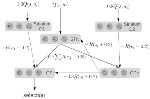
Figure 1. A model of action selection in the basal ganglia (Gurney et al., 2001). Each area stores N scalar values where N is the number of actions (for this diagram, N = 3). Inputs are Q(s, a): the utility values for each action, given the current state. The values affect each other by performing the computations shown on each connection (where R is the ramp function), and adding together all their inputs. Given a set of Q-values for input, the output y should be zero for the action with the largest Q-value, and positive for the other actions.
The connections between components define particular calculations, as indicated, where R is the ramp function. For a fixed input, the output y will converge to a set of values, with one value at (or near) zero, and the others positive. Importantly, this model will work for a very broad range of input Q-values and hundreds of actions. It should also be noted that this model converges very quickly (generally tens of iterations). A more complete discussion of the dynamics and capabilities of this model can be found elsewhere (Gurney et al., 2001).
We base our work on this model for three reasons. First, it provides precise information about the values being stored in the different areas of the basal ganglia, and the computations that are needed. Second, the activity of various parts of the model correlate well to the patterns of activity seen in the basal ganglia of rats in various conditions (Gurney et al., 2001). Third, the connections used in the model match well with the real basal ganglia. Striatal D1 neurons project primarily to GPi, and are known as the “direct” pathway. Striatal D2 neurons project primarily to GPe, which then connects to both the STN and the GPi, forming the “indirect” pathway. The STN also projects directly to the GPi, forming the “hyper-direct” pathway.
Furthermore, all of these connections are inhibitory, except for the ones from the STN which are excitatory. This fact is reflected in the model via the signs of the calculations performed in the equations: x is always added, and u, v, and z are always subtracted. All of the inhibitory connections are also highly selective in the basal ganglia: connections from one group of neurons tend to only affect a small group of neurons in the next component. This is also seen in the equations, as z1 affects x1, but not x2. Conversely, the excitatory connections from the STN are very broad, affecting large areas of their target components. This is again reflected in the equations, as x1 will affect all of z1, z2, z3, and so on. Indeed, the only major connectivity in the basal ganglia which is not covered by this model is that medium spiny neurons with dominant D1 receptors have been found to project to the GPe as well as the GPi (Parent et al., 2000). We thus feel that this model is a good starting point for constructing a more realistic spiking neuron model that respects the neurological constraints of the basal ganglia.
Materials and Methods
Our goal is to produce a computational model of behavior learning that uses realistic spiking neurons in a neurologically plausible manner. This requires the specification of a model of individual neurons, their connectivity, and how the strengths of those connections change over time.
Spiking Neurons
There are an extremely wide variety of models of individual neurons, depending both on the type of neuron and the amount of detail that is desired. The techniques we use here will work for any choice of neural model, but for simplicity we use the leaky-integrate-and-fire (LIF) neuron. This is widely used since not only is it a limiting case of more complex models such as the Hodgkin–Huxley model (Partridge, 1966), but it is also flexible enough to be an excellent approximation of a wide variety of neural models (Koch, 1999).
The dynamics of the LIF neuron model are given in Eq. 1. The voltage V changes in response to the input current I, and is dependent on the resistance R and capacitance C of the neuron. The product RC is known as the membrane time constant τRC and is a widely studied physiological value. For neocortical neurons, it is approximately 20 ms (McCormick et al., 1985; Plenz and Kitai, 1998) and for medium spiny neurons it has been found to be 13 ± 1 ms. These values are used in our model, for the corresponding neurons. We also note that C merely scales the input, and so can be ignored for the purposes of describing the model’s behavior.

An LIF neuron model generates a spike when its voltage V crosses a threshold. The voltage is then reset to its initial value, and held there for a fixed amount of time τref (the neuron’s refractory period). This is generally on the order of a few milliseconds. Given a fixed input current I, adjusting the two parameters τRC and τref results in changes to the neuron’s firing rate.
In real neurons, when a spike occurs neurotransmitter is released, affecting the flow of ions at the synapse. This is modeled by injecting current into the post-synaptic neuron whenever a spike occurs. This current injection, however, is not instantaneous. Instead, its effect is dependent on the neurotransmitter receptors and how quickly the neurotransmitter is reabsorbed by the pre-synaptic neuron. This neurotransmitter re-uptake rate τS widely varies for different neurotransmitters and neuron types, from hundreds of milliseconds for neocortical NMDA-type glutamate receptors (Flint et al., 1997) to 2 ms for AMPA-type glutamate receptors (Spruston et al., 1995; Smith et al., 2000). We model the post-synaptic current resulting from a spike via Eq. 2. For the excitatory connections in the basal ganglia (from STN to GPi and GPe), we use AMPA receptors with τS = 2 ms (Spruston et al., 1995). For the inhibitory connections (all others), we use GABA with τS = 8 ms (Gupta et al., 2000).

It should be noted that, while we are using simple LIF neurons in this model, the techniques we describe can also be used for more complex neural models. For example, we are currently investigating the effects of using the Gruber et al. (2003) model of medium spiny neurons, which exhibit bistability modulated by the level of dopamine.
Representation
In the basic basal ganglia action selection model discussed in Section “Action Selection Without Spikes,” numerical values are represented in the various different components. A standard practice in non-spiking neural models is to simply assume that each value is represented by one “neuron” in the model, so if there were three actions then there would be three neurons in each component, representing the three values. The activity of this neuron would be a single numerical value – perhaps the average level of activity of that neuron. However, when modeling using spiking neurons, a more nuanced approach is necessary, using a population of neurons to represent the value. While this might be done by simply assuming that all the neurons in that population are identical and that the average firing rate over all the neurons represents the value, this approach does not match what is observed in the brain.
Instead, we note that real neurons in the sensory and motor systems exhibit a wide variety of tuning curves when representing a single value. That is, given a set of neurons which fire quickly for a strong stimulus and slowly for a weak stimulus, the actual firing rates for these neurons will vary considerably, as in Figure 2. We achieve this in our model by adding two new parameters to each neuron: a fixed background input current Ibias and a fixed neuron gain factor α, which scales the neurons’ inputs. These values are randomly chosen to produce a highly heterogeneous population of neurons. The input current I is thus given by Eq. 3, where x is the value being represented.
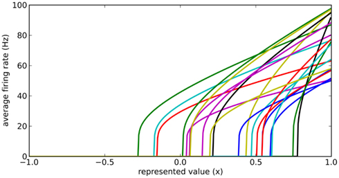
Figure 2. Typical randomly generated tuning curves for a population of 20 neurons. Each neuron has a different gain and background current, resulting in a different firing rate when representing the same value x.

Importantly, by adjusting the distributions of the gain and background current, different groups of neurons can have different maximum and background firing rates. For example, to model medium spiny neurons in the striatum, we choose Ibias to be slightly negative to give a background firing rate near zero, and the gain α to be such that the maximum current (occurring when x = 1) provides a firing rate between 40 and 60 Hz.
Computation
Here we adopt the spiking network construction method called the neural engineering framework (NEF; Eliasmith and Anderson, 2003). In this section we focus on the second principle of the framework, which provides a method for analytically determining connection weights to compute arbitrary functions in such networks. In particular, we derive a special case of this method that is sufficient to capture the computations needed for this basal ganglia model.
In the basal ganglia action selection model presented by Gurney et al. (2001), particular scalar computations must be performed between areas of the basal ganglia. For example, the population of neurons in GPe representing zi needs to have a value based on the values stored in STN and the striatum as per Eq. 4 [where R(x) is the ramp function, vi is the value represented by the ith group of striatal D2 neurons, and xi is the value represented by the ith group of STN neurons]. This must be accomplished entirely via the synaptic connections between these groups of neurons.

The idea here is to create connections between these groups such that the total input current to the individual neurons in the population corresponds to our desired input current as per Eq. 3. To simplify this task, we note that Eq. 3 is linear. This means that we could cause the neurons to represent y + z by having two sets of inputs: one for y and one for z, as in Eq. 5.

This allows us to break down the complex calculation in Eq. 4 into its linearly separable components. If we find connection weights that will compute those individual components, we can then simply combine all of them to arrive at connection weights that will compute the overall function. The basic component needed for computing all of the operations in the action selection model is given in Eq. 6, where b is a constant, R(x) is the ramp function, and x is a value represented by some other group of neurons.

To find these connection weights between the pre-synaptic population representing x and the post-synaptic population representing y, consider the neuron tuning curves shown in Figure 2. These show the firing rates of individual neurons for different values of x. Since each spike on a given connection produces roughly the same amount of input current, we can think of a synaptic connection strength as a scaling factor that converts a tuning curve into input current. What we want, then, is to take the tuning curves from Figure 2, scale each one by a different amount di, and add them together to produce the function given in Eq. 6. These scaling factors di then give us the synaptic connection weights ωij between the two neural populations, as shown in Eq. 7, where ai is the activity of the ith neuron in the pre-synaptic population.

Our final step is to find the scaling factors di that will take the set of tuning curves and find the best way to approximate the desired function f(x). This is a well-defined least-squares minimization problem: we want to minimize the error E between f(x) and the weighted sum of the tuning curves a(x), as in Eq. 8. This is done by the standard method of taking the derivative and setting it equal to 0.
To solve this for dj, we convert to matrix notation, arriving at Eq. 9.
The vector d has one element for each neuron, which is that neuron’s appropriate scaling factor. Since ωij = αjdi (Eq. 7), this result allows us to find synaptic connection weights that will approximate any desired function, given a set of neurons with varying tuning curves. For this particular case, Figure 3 shows that even just three neurons can be used to closely approximate the R(x − b) function needed here. As the number of neurons used increases, the error decreases (Figure 4). Furthermore, networks resulting from this method are highly robust to random noise and destruction of individual neurons (Eliasmith and Anderson, 2003).
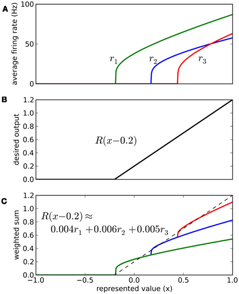
Figure 3. Approximating a desired function by weighted sums of tuning curves. The three neurons in (A) fire at different rates when representing different x values. To approximate the desired function shown in (B), we weight each tuning curve ri by a different value di and add them together (C). These weighting factors di can be calculated with Eq. 9 and used to find synaptic connection weights with Eq. 7.
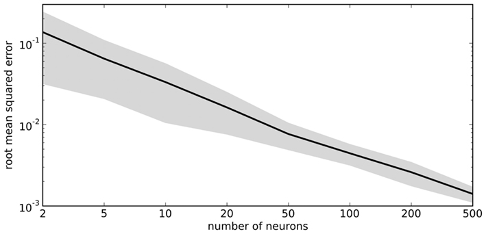
Figure 4. Accuracy of approximating R(x − 0.2) using varying numbers of random neural tuning curves. Gray area shows ±1 SD of 100 samples for each point.
The NEF methodology generalizes to representing multiple dimensions, functions, and vector fields, as well as other neuron models and more complex non-linear functions (Eliasmith and Anderson, 2003). It has been used to construct large-scale models of inductive reasoning (Rasmussen and Eliasmith, 2011), serial recall (Choo and Eliasmith, 2010), path integration (Conklin and Eliasmith, 2005), and many others. It provides a general method for building models with realistic spiking neurons and directly solving for connection weights that will compute particular desired functions. As such, it is ideally suited for converting models such as the basal ganglia action selection model into a more realistic detailed neural simulation.
Action Selection
Given the neural representation approach described in Section “Representation” and the ability to solve for connection weights to compute particular functions given in Section “Computation,” we can implement the complete action selection model from Gurney et al. (2001) using spiking neurons. We replace each variable in the original model with a population of 40 LIF neurons with randomly selected background currents (Ibias) and gains (α), producing a wide variety of tuning curves (as per Figure 2). We compute connection weights between populations using Eqs 7 and 9, such that the particular calculations in the original model are faithfully reproduced. The result is a spiking neuron model of action selection.
We can send input into this model by driving current into the striatal and STN neuron populations as per Eq. 3, and read the output from the spiking activity of the GPi neurons. Figure 5 shows that the model successfully selects the action with the highest utility, as does the original non-spiking model. However, since this is now a spiking model, we can also analyze other factors of its behavior, such as the amount of time needed for it to make this selection. This value will be dependent on the neurotransmitter time constants involved (see Eq. 2). As we have previously shown (Stewart et al., 2010b), the timing behavior of this model matches well to that of the rat basal ganglia, where it takes 14–17 ms for a change in activity in the cortex to result in a selection change in GPi (Ryan and Clark, 1991).
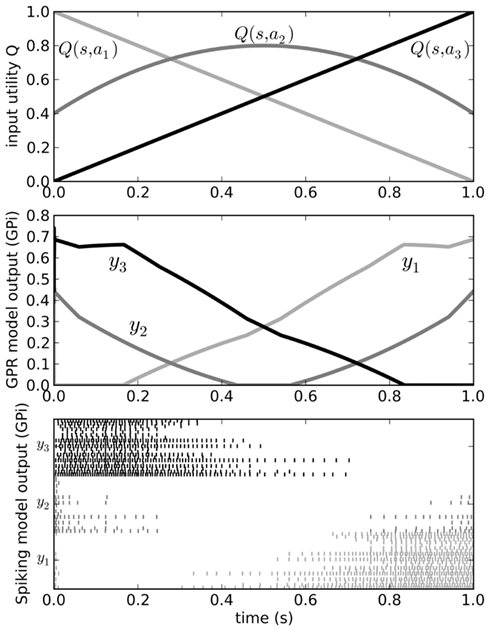
Figure 5. Behavior of the original Gurney et al. (2001) model (middle) for a varying input (top). Spiking output from the GPi neurons in our model is also shown (bottom). Varying input corresponds to changing the utilities Q of the three actions a1, a2, and a3 as the current state s changes over time. Since the output from the GPi is inhibitory, the neurons corresponding to the chosen action should stop firing when that action’s Q-value is larger than that of the other two.
State Representation
The components of the model so far are sufficient to allow us to take a set of utility values Q (the inputs to the basal ganglia model) and produce an output which identifies the largest of these inputs. However, for this to be a more complete model of action selection, we also need to compute these utility values themselves.
Utility values are generally based on a currently represented state. Our approach is to assume that this state is represented in the cortex, and the connections between the cortex and the basal ganglia compute the utility. To start this process, we need to define how state information is represented in cortex. We follow a similar approach as taken in Section “Representation,” but we generalize to multidimensional state. That is, we want to represent x where x is some vector of arbitrary length, rather than a single scalar value. As before, we have a large population of neurons, each of which has a randomly chosen gain and background current. However, since x is not a scalar, we multiply it by p, a randomly chosen state vector for each neuron, giving Eq. 10.

This vector p can be thought of as a preferred state vector: the state for which this particular neuron will be most active. The result is a highly distributed multidimensional state representation that produces firing patterns that match closely to those seen throughout sensory and motor cortex (e.g., Georgopolous et al., 1986). We discuss the implications of this method of representation in more detail elsewhere (Stewart et al., 2011; Eliasmith and Anderson, 2003).
Given this method of representing state, it would be possible to compute connection weights using Eq. 9, if we also knew the function Q mapping state to utility. We have used this approach in previous models, most recently in a model of the Tower of Hanoi task, where at each moment 1 of 19 different actions must be chosen, based on the current state (Stewart and Eliasmith, 2011). However, here we instead want to learn the utility based on reinforcement feedback from the environment.
Learning Action Utilities
Since the utility of different actions must be learned based on interaction with the environment, we need a learning rule that will adjust synaptic connections between cortex and basal ganglia. A standard approach to learning in neural networks is the delta rule, where the weight is changed based on the product of the activity of the pre-synaptic neuron and an error signal. For our model, we use a spike-based rule given in Eq. 11, where κ is a learning rate and e is an error term: the difference between the actual utility and the currently predicted utility (as before, ai is the activity of the pre-synaptic neuron, and αj is the gain of the post-synaptic neuron).

This is a local learning rule: all of the information used is available local to the synapse, and no synapse needs to communicate to other synapses. Furthermore, for ai and e we use the instantaneous measure of the level of neurotransmitter at the synapse, rather than any sort of long-term average firing rate, which would be difficult for the molecules at the synapse to estimate. It is a special case of a more general rule derived by MacNeil and Eliasmith (2011), and has been shown to be useful in a variety of supervised learning situations (Bekolay, 2011).
To make use of this rule, however, we need the error signal e. The simplest approach is to take the difference between the actual reward r received for performing action k and subtract the current estimate Q of the value for performing action k in the current state s, as shown in Eq. 12.

For our model, we take this prediction error calculation to be performed by the ventral striatum. This is a somewhat controversial statement, given that there are a broad range of proposed suggestions as to how reward, expected reward, and reward prediction error could be represented in the basal ganglia (see Schultz, 2006 for an overview). However, we do note that while some fMRI results show activation in the ventral striatum is more correlated to reward than to reward prediction error, it is also the case that the activation measured by fMRI is indicative of the neural inputs to an area, not the spiking behavior of the neurons in that area (Logothetis et al., 2001). This is consistent with our model.
We construct this component in the same manner as the other calculations: a group of neurons represents the error value and the connections to these neurons can be computed using Eqs. 7 and 9. For our model, we do not consider where the reward signal r comes from; rather we directly inject the appropriate current into the ventral striatum neurons using Eq. 3.
To model the effects of this reward prediction calculation, we need to convert the error signal e into a form that can be used by the synapses to adjust their connection strengths. It is widely believed that the neurotransmitter dopamine can modulate synaptic connection weights, and dopamine levels corresponding to reward prediction errors have been widely observed (e.g., Schultz et al., 1997). Dopamine is produced by neurons in the part of the basal ganglia known as the SNc, so we form corresponding connections from the ventral striatum to the SNc, using Eqs. 7 and 9 where f(x) = x (since we are merely passing information between these components, not performing any calculation). We then form connections back to the striatum [also using f(x) = x]. However, instead of having a spike in the SNc produce current that goes into the cells in the striatum, we have these connections merely affect the level of dopamine near those neurons, which we treat as e in Eq. 11. The result is a biologically plausible calculation of the required learning rule.
The effect of this system is that the output from the SNc neurons provides different levels of dopamine to the different neural groups representing the various actions in the striatum. This dopamine level e for each group indicates whether the currently predicted utility Q is too high or too low. Given the learning rule from Eq. 11, we can start with random connections between the cortex and basal ganglia, and over time the system should learn connection weights that make correct estimates of utility. The resulting model is shown in Figure 6.
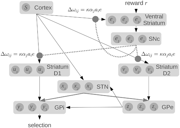
Figure 6. Our spiking model of reward-based learning and action selection in the cortex and basal ganglia. Dotted lines show dopaminergic connections from the substantia nigra pars compacta (SNc) which modulate the local synaptic strengths using the equations shown. Raw reward signal is input into the ventral striatum, which also computes an estimate of Q(s, a) using connections from the cortex. The difference between these values is fed to the SNc, which produces the error signal.
It should be noted that this model does not use a single, global dopamine signal. Instead, the neurons for different actions in the striatum will receive different levels of dopamine. While it is often assumed that dopamine levels are the same everywhere, Aragona et al. (2009) have shown that phasic dopamine levels vary across different regions of the striatum. Our approach of having the error signal broken down into prediction errors for each candidate action is not a standard interpretation in the field. However, we believe our model provides one possible interpretation of these results. Furthermore, there is considerable evidence that the strength of connections between cortex and striatum is modulated by the presence of dopamine, consistent with our learning rule (Calabresi et al., 2000).
Bandit Task
The bandit task is a standard experimental paradigm where the subject is given a choice between two or more actions, each of which results in rewards randomly drawn from a probability distribution specific to that action. The subject’s goal is to maximize the amount of reward it receives over time. Stated differently, the subject must determine which action’s associated probability distribution is the most rewarding in the long-term. The probability distributions may remain the same (static bandit task) or change over time (dynamic bandit task).
The number of possible actions determines the number of “arms” in the bandit task. This terminology results from one realization of the bandit task, in which the subject chooses to pull a lever on a slot machine with two or more levers (“arms”). Animal experiments are either done with lever presses or mazes with decision points.
We chose Kim et al.’s (2009) study of rats performing a dynamic two-armed bandit task to test our basal ganglia model. In this study, rats run a small maze with only one decision point, with two possible choices at that decision point. Each choice leads to a reward site with a certain probability of water reward. The probability of reward changed every 40 trials. Most importantly for our purposes, this study couples behavioral data with measurements of spiking activity in the striatum. This allows us to evaluate our model at both the behavioral level and the neural spiking level.
Results
To validate our model, we examined three different scenarios based on the rat bandit task described in the previous section. We start by replicating the experiment by Kim et al. (2009), and then examine whether the model continues to function when given more actions to choose between, or more states on which the decision can be based.
The Two-Arm Bandit Task
The model successfully replicates the rat behavior seen by Kim et al. (2009). Initially, the model chooses randomly between the two branches of the maze. During the first 40 trials, it gradually chooses the right side more and more often, as it receives a reward 63% of the time. After this block the rewards switch, and the model learns to prefer the left branch. In the final two blocks, these rewards switch again. Average behavior over 200 simulated rats is shown in Figure 7, along with the a sample empirical data and the closest fitting model data for that run (RMSE = 0.182).
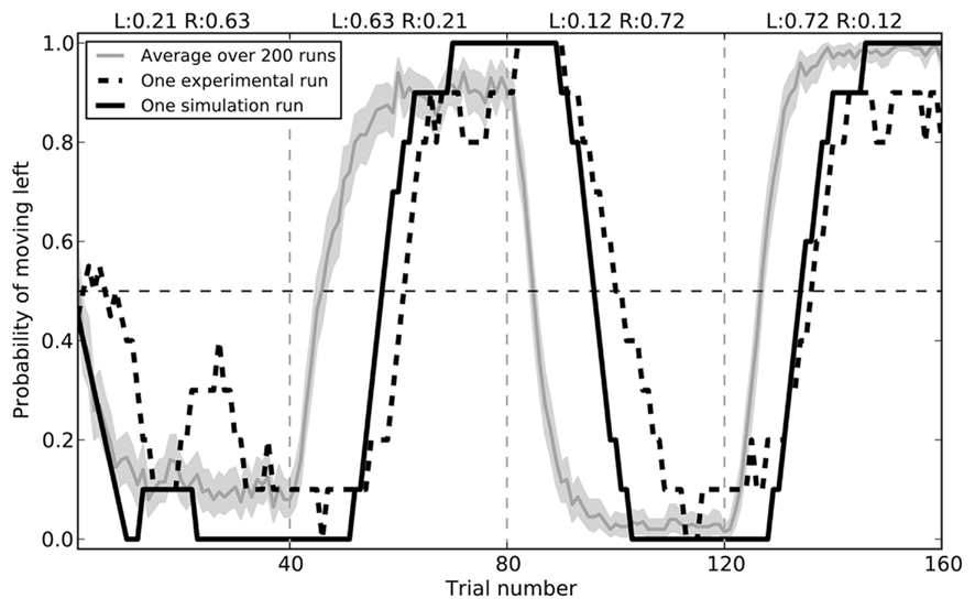
Figure 7. Model performance compared to sample empirical data from Kim et al. (2009). Black lines show a single run, plotting the proportion of time the rat or the model chose to go left over 160 trials, averaged with a 10-trial window. The gray area gives the mean performance of the model over 200 runs, with 95% bootstrap confidence interval.
While the rats performed the choice experiment, spiking activity in the ventral striatum was also measured. This activity was shown to be sensitive to the decision being made. In Figure 8, we compare the activity seen in the rats (Kim et al., 2009) to that seen in the model for decisions involving turning to the left. The activity of the model matches that of the rats.
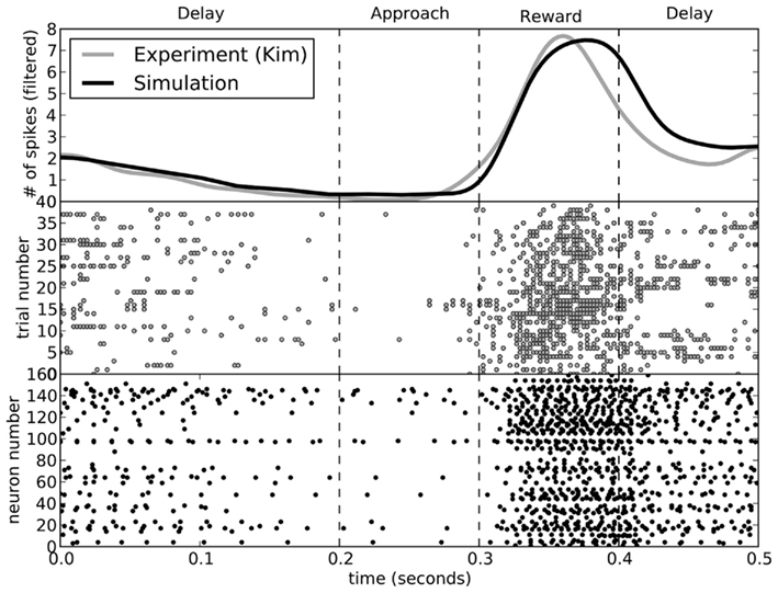
Figure 8. A comparison of spike patterns in the ventral striatum of the rat (from Kim et al., 2009) and our model. The top area shows spike counts, with a Gaussian filter of 15 ms. All data is from runs where the rat (or model) turned to the left.
To quantify the accuracy of the model, Figure 9 shows this same data plotted with 95% bootstrap confidence intervals. In the bottom of Figure 9, we compute the maximum likely difference (MLD; Stewart and West, 2010) between the model and rat data. The black line shows the average difference, and the gray area gives the 95% confidence interval of the difference between the models. Whenever they gray area touches zero, the model data is not statistically significantly different from the empirical data (p > 0.05). This indicates that there is a small discrepancy between the model and the rats at the end of the reward phase. At that time (t = 0.4), the error in terms of number of spikes is between 1 and 5. For the rest of the time, the model is not statistically different from the empirical data. However, this does not mean that the model is a perfect predictor of performance – as with any model, if more data were gathered, then we would eventually find some level of discrepancy. However, the MLD measure is shown as the top of the gray area and provides an upper bound on the prediction error from the model (with 95% confidence). This indicates that the model usually produces predictions that we can be 95% confident are within two spikes of the actual measurement, except for during the reward phase where the error may increase up to 5 (or possibly stay as low as 1). More empirical measurements are needed to further compute the accuracy of this model.
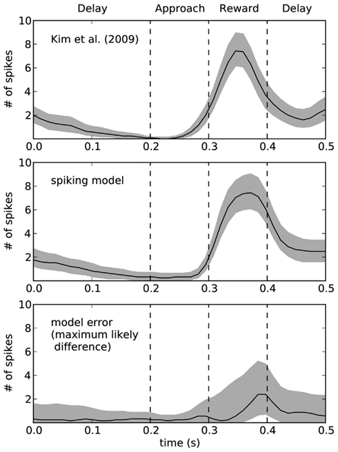
Figure 9. Ninety five percentage bootstrap confidence intervals for the spike counts of the model and the empirical data. Bottom graph shows the difference between these models, where the black line is the average difference and the top of the gray area shows the maximum likely difference (MLD; Stewart and West, 2010). MLD indicates that we can be 95% confident that the model produces behavior that is accurate to within this value, thus placing an upper bound on the error in the model. The bottom of the gray area indicates the lower bounds on the model error, such that whenever the gray area does not include zero we can find a statistically significant difference between the model and the empirical data.
The Three-Arm Bandit Task and Multiple States
The two-arm bandit task is extremely simple. There is only a single state s, and there are only two choices that can be made. To determine if our model can handle more complex situations, we made two modifications to the experimental situation. The first of these was to simply add a third action (choosing a center path, rather than left or right), demonstrating that the action selection system can learn to successfully choose between three separate actions (Figure 10).
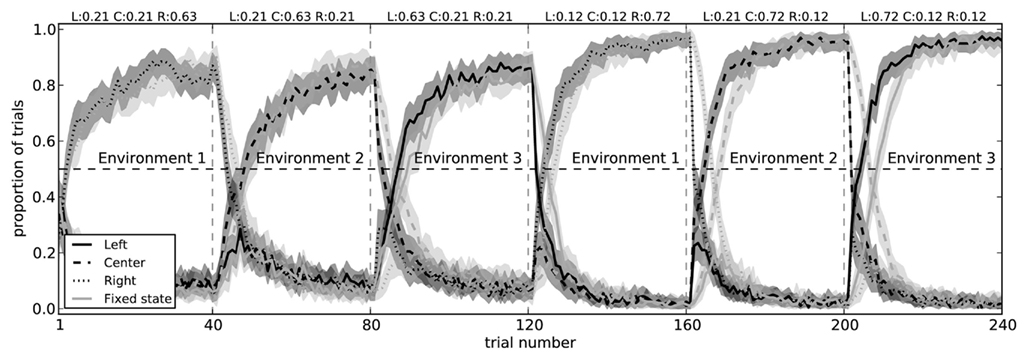
Figure 10. Model performance on a three-arm bandit task with fixed state information (light gray) and with state that changes for each block (dark gray). In both conditions, the model successfully learns to choose the action which most often gives it a reward. When the state information is fixed (i.e., when the pattern of spikes in the cortex does not change to indicate which of the three environments it is in), the model takes longer to switch actions. Shaded areas are 95% bootstrap confidence intervals over 200 runs.
The other manipulation we added to is to have different states. In the original experiment, every time the rat made a choice, it was in the same state. This was represented in the model by having the cortex neurons firing with a particular pattern, caused by choosing a random vector x to represent that state, and injecting current into each neuron using Eq. 10. This resulted in each neuron firing with a different pattern (since each neuron had a different preferred state p, gain α, and background current Ibias), forming a distributed representation of that state. Thus, during the first 40 trials in the original task (Figure 7), the rat learned to associate that state with turning right. In the next 40 trials, it then had to change that association because it was suddenly being rewarded more often for turning left instead.
While Figure 7 shows that the model is capable of changing a learned utility value, we also want to show that the model can learn that different states have different utilities for the different actions. That is, Q(s1,a1) may be different than Q(s2,a1). We test this by creating three separate randomly chosen vectors for the states, and having the input current (Eq. 10) to the cortex neurons change depending on which state the agent is in. This can be thought of as having three visually distinct environments, and in environment 1 the rat is most rewarded for turning right, in environment 2 it is most rewarded for the center, and in environment 3 it should choose the left.
Importantly, when the state information allows the model to distinguish which choice is best, it does not need to unlearn previous utility values. That is, instead of being surprised when the rewards suddenly change between blocks, the state representation also changes. As expected, the model is faster at switching to the correct action when it has state information, as opposed to the condition where there is a fixed state for all blocks (Figure 10). This indicates it is successfully learning that Q(s1,a1) ≠ Q(s2,a1).
Stopping Learning
To further test our model, we can observe its actions with learning disabled. That is, we can train it in two separate environments where in each environment the neurons in cortex represent a different randomly chosen state vector. For environment 1, choosing to turn right is rewarded 72% of the time, and choosing to turn left is rewarded 12% of the time. For environment 2, the probabilities are swapped. These rewards are the same as those in the final block of the rat experiments. Figure 11 shows what happens when the model is exposed to 40 trials of the first environment followed by 40 trials of the second environment, and then has learning disabled. The model is able to successfully respond correctly in the second environment, but is only slightly above chance at the first environment.
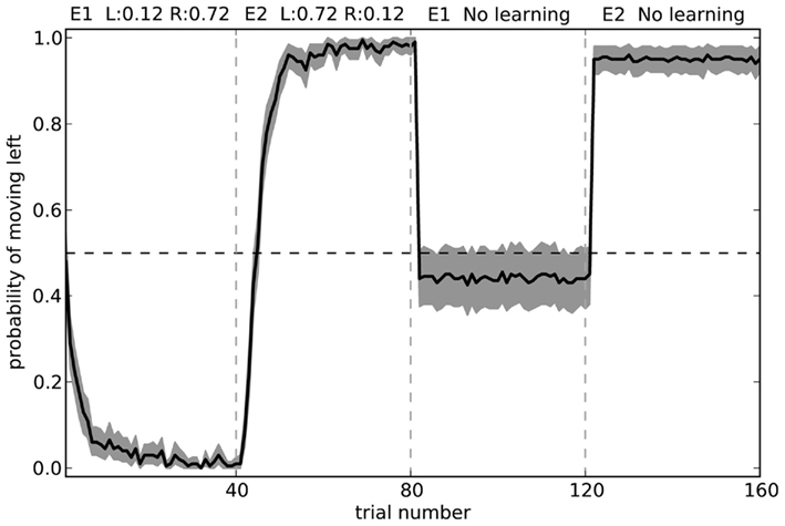
Figure 11. Model performance when learning is turned off after the first 80 trials. Shaded area shows 95% bootstrap confidence intervals over 200 runs. A different randomly chosen state vector is used for each of the two environments.
The fact that the model forgets what to do in the first environment is the common “interference” problem of any neural-based learning system. We can improve its performance by changing the training regime to alternate more quickly. Figure 12 shows the model performance when exposed to the same number of total trials in each environment, but alternating every 10 blocks. Here, the model is considerably more accurate.
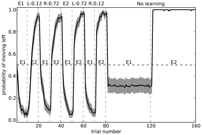
Figure 12. Model performance when learning is turned off after the first 80 trials. During learning, the environment is swapped every 10 trials, rather than every 40 as in Figure 11. Shaded area shows 95% bootstrap confidence intervals over 200 runs. A different randomly chosen state vector is used for each of the two environments.
Discussion
The model we have presented here provides a mechanistic explanation of many aspects of reward-based decision making via the basal ganglia. The model consists entirely of LIF neurons whose parameters have been matched to the neurologically observed values in corresponding areas of the basal ganglia. These neurons produce realistic heterogeneous firing patterns, and we have shown that the spike pattern seen in the ventral striatum of rats performing a two-arm bandit task closely matches that seen in our model. The connections between the various groups of neurons in our model correspond to the major known connections in the basal ganglia and cortex, including whether they are excitatory or inhibitory, their neurotransmitter re-absorption rate, and how broad or selective their connections are. We are aware of no other model that provides this level of neurological detail and is capable of flexibly learning to select different actions in different states based on reward. While non-spiking models exist that can produce similar behavior, they achieve this at the cost of abstracting away details that can help constrain models. Furthermore, our spike-based approach opens the door to using highly detailed neural models, such as Gruber et al.’s (2003) medium spiny neuron model.
This model does not, of course, explain all of decision making. While we allow for the representation of arbitrarily complex states in cortex, we make no claims about how the brain develops and maintains these representations. The only assumption we make is that different states correspond to different patterns of activation in cortex. However, our model does explain how the brain can start with an initially random set of connections between the cortex and the striatum, and then use the local level of dopamine to modulate the strength of these connections to compute the expected utility, Q, of performing different actions given this state. Furthermore, we show how neurons in the ventral striatum and SNc can use a reward input to correctly adjust that level of dopamine. We do not consider, however, how this reward input is generated. Once the utility is computed in the striatum, we use our previously published spiking model of the rest of the basal ganglia (based on the non-spiking model of Gurney et al., 2001) to select one particular action. It should also be noted that we do not consider here how the connections in the basal ganglia develop – all learning in our model occurs between the cortex and striatum, leaving the connections within the basal ganglia to be computed (Eqs. 7 and 9).
Parameter Fitting
A general problem with all computational modeling is the issue of parameter fitting. However, since we are using a spiking neuron model, the vast majority of our parameters can be set based on known neurological measurements. This provides us with most of the neural values in our model (τRC, τref, τS, Ibias, α). For the models presented here, we use τRC = 20 ms, τref = 2 ms, τS = 2 ms for AMPA and 8 ms for GABA, and randomly vary Ibias and α to create heterogeneous populations with different mean and maximum firing rates for different regions of the brain. While these values do affect the temporal performance of the basic basal ganglia model (Stewart et al., 2010b), they were not tuned in any way for the results shown here.
The learning rate κ does have a significant effect on the performance of this model. As expected, since it affects how quickly the synaptic connections change strength, its behavioral effect is that it leads to faster transitions when the reward structure changes. In future work, we will constrain this parameter value through both behavioral and neurological data, but in this model we used κ = 1.0 × 10⁻⁷, since values between 1.0 × 10⁻⁷ and 2.0 × 10⁻⁶ have been previously shown to work well with this learning rule for other tasks (Bekolay, 2011). No parameter fitting was performed for the results given here.
For the remaining parameters, we have not yet thoroughly explored the effects of changing these parameters. In this model, we used 40 neurons per population because previous work with the basal ganglia model indicated that accuracy decreased with less than 35 neurons, but no performance effects were seen for larger values. The initial connection strengths between cortex and striatum ωij were set randomly with a uniform distribution between −0.0001 and 0.0001, but as long as these are sufficiently small, the model performs as seen here.
It should also be noted that the gain α on neurons in the ventral striatum has the effect of scaling the overall firing rate of those neurons, but generally has no other effect (although as this value is reduced, more neurons are needed in a group to produce accurate decision making). As previously mentioned, the range of values for the neurons in this area was tuned to match the maximum firing rates seen in this area, so this has the effect of scaling along the y-axis in Figure 8. However, this parameter does not affect the overall shape of that graph.
Limitations
While our model is more physiologically accurate than other learning models of this type, there is certainly room for improvement. More detailed models of the medium spiny neuron in the striatum do exist (Gruber et al., 2003), and we are in the process of integrating them into our model. Furthermore, a more detailed model of the process whereby dopamine affects the long-term strength of a synapse could modify our learning rule (Eq. 11) and potentially provide neurological constraints on the learning rate parameter κ.
One major component of decision making and reinforcement learning that is not included in the current model is associating states that occur sequentially in time, a problem typically solved by temporal-difference learning methods. Our reward prediction equation, Eq. 12, is notably missing an estimate of the next state’s value. This is a difficult quantity to make available to a system that operates continuously in time, as ours does. One approach to including this would be to add a prediction module that predicts future states, actions, and their associated Q-values. Potjans et al.’s (2009) spiking actor–critic model solves this by using a slow activity trace of the Q-values, such that there is a critical point in time in which the model represents the current Q-value and the previous Q-value. We are currently investigating using this idea in our model.
A feature seen in the biological basal ganglia that we do not currently model is the reward system’s ability to make precise temporal predictions. As shown in Schultz’s (1997) original experiments, the activity of dopamine neurons changes depending on the precise time that a reward is predicted. Our current model is insensitive to the time that a reward is delivered (or not delivered). Incorporating this may come as a result of the network dynamics resulting from incorporating linking together sequentially occurring states, or it may require a more reasoned approach to detecting the time elapsed since a stimulus. We believe this sort of timing system may help reduce the discrepancy between the model and the empirical data shown in Figure 9.
Conclusion
The model we have presented here is a generic neurologically accurate spiking reward-based decision making system closely modeled on the mammalian basal ganglia. While we have previously used the core action selection aspect of the basal ganglia model to produce complex models of planning and problem solving (Stewart and Eliasmith, 2011; Stewart et al., 2010a,b), our new model successfully adds the ability to learn the utility of various actions in different contexts based on external rewards, using a dopamine-based prediction error signal. The results presented here show that the model is capable of learning simple forced choice tasks and producing accurate predictions of spike patterns in the ventral striatum. Our ongoing project is to further evaluate the predictions of this model and investigate its performance in more complex tasks.
Conflict of Interest Statement
The authors declare that the research was conducted in the absence of any commercial or financial relationships that could be construed as a potential conflict of interest.
Acknowledgments
This research was supported by funding from the SHARCNET Research Fellowship Program, the Natural Sciences and Engineering Research Council of Canada, the Canada Foundation for Innovation, the Ontario Innovation Trust, and the Canada Research Chairs program.
References
Aragona, B., Day, J., Roitman, M., Cleaveland, N., Wightman, R. M., and Carelli, R. (2009). Regional specificity in the real-time development of phasic dopamine transmission patterns during acquisition of a cue-cocaine association in rats. Eur. J. Neurosci. 30, 1889–1899.
Barto, A. G. (1995). “Adaptive critics and the basal ganglia,” in Models of Information Processing in the Basal Ganglia, eds J. C. Houk, J. Davis, and D. Beiser (Cambridge: MIT Press), 215–232.
Bekolay, T. (2011). Learning in Large-Scale Spiking Neural Networks. Masters thesis, Computer Science, University of Waterloo, Waterloo.
Calabresi, P., Gubellini, P., Centonze, D., Picconi, B., Bernardi, G., Chergui, K., Svenningsson, P., Fienberg, A. A., and Greengard, P. (2000). Dopamine and cAMP-regulated phosphoprotein 32 kDa controls both striatal long-term depression, and long-term potentiation, opposing forms of synaptic plasticity. J. Neurosci. 20, 8443–8451.
Choo, F., and Eliasmith, C. (2010). “A spiking neuron model of serial-order recall,” in Proceding of the 32nd Annual Conference of the Cognitive Science Society, eds R. Cattrambone, and S. Ohlsson (Austin, TX: Cognitive Science Society), 2188–2193.
Conklin, J., and Eliasmith, C. (2005). An attractor network model of path integration in the rat. J. Comput. Neurosci. 18, 183–203.
Eliasmith, C., and Anderson, C. H. (2003). Neural Engineering: Computation, Representation, and Dynamics in Neurobiological Systems. Cambridge, MA: MIT Press.
Flint, A. C., Maisch, U. S., Weishaupt, J. H., Kriegstein, A. R., and Monyer, H. (1997). NR2A subunit expression shortens NMDA receptor synaptic currents in developing neocortex. J. Neurosci. 17, 2469–2476.
Frank, M. J. (2005). Dynamic dopamine modulation in the basal ganglia: a neurocomputational account of cognitive deficits in medicated and non-medicated Parkinsonism. J. Cogn. Neurosci. 17, 51–72.
Georgopolous, A. P., Schwartz, A., and Kettner, R. E. (1986). Neuronal population coding of movement direction. Science 260, 47–52.
Gruber, A. J., Solla, S. A., Surmeier, D. J., and Houk, J. C. (2003). Modulation of striatal single units by expected reward: a spiny neuron model displaying dopamine-induced bistability. J. Neurophysiol. 90, 1095–1114.
Gupta, A., Wang, Y., and Markram, H. (2000). Organizing principles for a diversity of GABAergic interneurons and synapses in the neocortex. Science 287, 273–278.
Gurney, K., Prescott, T., and Redgrave, P. (2001). A computational model of action selection in the basal ganglia. Biol. Cybern. 84, 401–423.
Humphries, M., Stewart, R., and Gurney, K. (2006). A physiologically plausible model of action selection and oscillatory activity in the basal ganglia. J. Neurosci. 26, 12921–12942.
Izhikevich, E. M. (2007). Solving the distal reward problem through linkage of STDP and dopamine signaling. Cereb. Cortex 17, 2443–2452.
Joel, D., Niv, Y., and Ruppin, E. (2002). Actor-critic models of the basal ganglia: new anatomical and computational perspectives. Neural Netw. 15, 535–547.
Kim, H., Sul, J. H., Huh, N., Lee, D., and Jung, M. W. (2009). Role of striatum in updating values of chosen actions. J. Neurosci. 29, 14701–14712.
Koch, C. (1999). Biophysics of Computation: Information Processing in Single Neurons. New York, NY: Oxford University Press.
Logothetis, N. K., Pauls, J., Augath, M., Trinath, T., and Oeltermann, A. (2001). Neurophysiological investigation of the basis of the fMRI signal. Nature 412, 150–157
MacNeil, D., and Eliasmith, C. (2011). Fine-tuning and stability of recurrent neural networks. PLoS ONE 6, e22885. doi: 10.1371/journal.pone.0022885
McCormick, D. A., Connors, B. W., Lighthall, J. W., and Prince, D. A. (1985). Comparative electrophysiology of pyramidal and sparsely spiny stellate neurons of the neocortex. J. Neurophysiol. 54, 782–806.
Parent, A., Sato, F., Wu, Y., Gauthier, J., Lévesque, M., and Parent, M. (2000). Organization of the basal ganglia: the importance of axonal collateralization. Trends Neurosci. 23, S20–S27.
Partridge, L. (1966). A possible source of nerve signal distortion arising in pulse rate encoding of signals. J. Theor. Biol. 11, 257–281.
Plenz, D., and Kitai, S. (1998). Up and down states in striatal medium spiny neurons simultaneously recorded with spontaneous activity in fast-spiking interneurons studied in cortex–striatum–substantia nigra. J. Neurosci. 18, 266–283.
Potjans, W., Morrison, A., and Diesmann, M. (2009). A spiking neural network model of an actor-critic learning agent. Neural Comput. 21, 301–339.
Prescott, T., González, F., Gurney, K., Humphries, M., and Redgrave, P. (2006). A robot model of the basal ganglia: behavior and intrinsic processing. Neural Netw. 19, 31–61.
Rangel, A., Camerer, C., and Montague, P. R. (2008). A framework for studying the neurobiology of value-based decision making. Nat. Rev. Neurosci. 9, 545–556.
Rasmussen, D., and Eliasmith, C. (2011). A neural model of rule generation in inductive reasoning. Top. Cogn. Sci. 3, 140–153.
Redgrave, P., Prescott, T., and Gurney, K. (1999). The basal ganglia: a vertebrate solution to the selection problem? Neuroscience 86, 353–387.
Ryan, L., and Clark, K. (1991). The role of the subthalamic nucleous in the response of globus pallidus neurons to stimulation of the pre-limbic and agranular frontal cortices in rats. Exp. Brain Res. 86, 641–651.
Schultz, W. (2006). Behavioral theories and the neurophysiology of reward. Annu. Rev. Psychol. 57, 87–115.
Schultz, W., Dayan, P., and Montague, P. R. (1997). A neural substrate of prediction and reward. Science 275, 1593–1599.
Shouno, O., Takeuchi, J., and Tsujino, H. (2009). A spiking neuron model of the basal ganglia circuitry that can generate behavioral variability. Adv. Behav. Biol. 58, 191–200.
Smith, A. J., Owens, S., and Forsythe, I. D. (2000). Characterisation of inhibitory and excitatory postsynaptic currents of the rat medial superior olive. J. Physiol. 529, 681–698.
Spruston, N., Jonas, P., and Sakmann, B. (1995). Dendritic glutamate receptor channel in rat hippocampal CA3 and CA1 pyramidal neurons. J. Physiol. 482, 325–352.
Stewart, T. C., Bekolay, T., and Eliasmith, C. (2011). Neural representations of compositional structures: representing and manipulating vector spaces with spiking neurons. Conn. Sci. 22, 145–153.
Stewart, T. C., and West, R. (2010). Testing for equivalence: a methodology for computational cognitive modelling. J. Artif. Gen. Intel. 2, 69–87.
Stewart, T.C., Choo, X., and Eliasmith, C. (2010a). “Symbolic reasoning in spiking neurons: a model of the cortex/basal ganglia/thalamus loop,” in Proceeding of the 32nd Annual Meeting of the Cognitive Science Society, eds R. Cattrambone, and S. Ohlsson (Austin, TX: Cognitive Science Society), 1100–1105.
Stewart, T.C., Choo, X., and Eliasmith, C. (2010b). “Dynamic behaviour of a spiking model of action selection in the basal ganglia,” in Proceedings of the 10th International Conference on Cognitive Modeling, eds D. Salvucci, and G. Gunzelmann (Philadelphia, PA: Drexel University), 235–240.
Stewart, T.C., and Eliasmith, C. (2011). “Neural cognitive modelling: a biologically constrained spiking neuron model of the Tower of Hanoi task,” in Proceeding of the 33rd Annual Meeting of the Cognitive Science Society, eds L. Carlson, C. Hölscher, and T. Shipley (Austin, TX: Cognitive Science Society), 656–661.
Keywords: basal ganglia, ventral striatum, reinforcement learning, two-armed bandit, neural engineering framework
Citation: Stewart TC, Bekolay T and Eliasmith C (2012) Learning to select actions with spiking neurons in the basal ganglia. Front. Neurosci. 6:2. doi: 10.3389/fnins.2012.00002
Received: 01 October 2011; Accepted: 04 January 2012;
Published online: 31 January 2012.
Edited by:
Leendert Van Maanen, University of Amsterdam, NetherlandsReviewed by:
Michael X. Cohen, University of Amsterdam, NetherlandsBruno B. Averbeck, National Institute of Mental Health, USA
Copyright: © 2012 Stewart, Bekolay and Eliasmith. This is an open-access article distributed under the terms of the Creative Commons Attribution Non Commercial License, which permits non-commercial use, distribution, and reproduction in other forums, provided the original authors and source are credited.
*Correspondence: Terrence C. Stewart, Centre for Theoretical Neuroscience, University of Waterloo, 200 University Avenue West, Waterloo, ON, Canada N2L 3G1. e-mail: tcstewar@uwaterloo.ca