Spike sorting of heterogeneous neuron types by multimodality-weighted PCA and explicit robust variational Bayes
- 1Laboratory for Neural Circuit Theory, RIKEN Brain Science Institute, Wako, Japan
- 2Brain Science Institute, Tamagawa University, Machida, Japan
This study introduces a new spike sorting method that classifies spike waveforms from multiunit recordings into spike trains of individual neurons. In particular, we develop a method to sort a spike mixture generated by a heterogeneous neural population. Such a spike sorting has a significant practical value, but was previously difficult. The method combines a feature extraction method, which we may term “multimodality-weighted principal component analysis” (mPCA), and a clustering method by variational Bayes for Student's t mixture model (SVB). The performance of the proposed method was compared with that of other conventional methods for simulated and experimental data sets. We found that the mPCA efficiently extracts highly informative features as clusters clearly separable in a relatively low-dimensional feature space. The SVB was implemented explicitly without relying on Maximum-A-Posterior (MAP) inference for the “degree of freedom” parameters. The explicit SVB is faster than the conventional SVB derived with MAP inference and works more reliably over various data sets that include spiking patterns difficult to sort. For instance, spikes of a single bursting neuron may be separated incorrectly into multiple clusters, whereas those of a sparsely firing neuron tend to be merged into clusters for other neurons. Our method showed significantly improved performance in spike sorting of these “difficult” neurons. A parallelized implementation of the proposed algorithm (EToS version 3) is available as open-source code at http://etos.sourceforge.net/.
Introduction
Since a vast number of neurons are simultaneously active in the brain, the analyses of action potentials (spikes) of multiple neurons are crucial for uncovering the principle of brain computation. Electrical activity of multiple neurons can be recorded with high temporal resolution using electrodes located outside of neural cell bodies (O'Keefe and Recce, 1993; Wilson and McNaughton, 1993; Fynh et al., 2007). The extracellularly recorded data contains spikes of many neurons surrounding the tip of electrodes, and all spike-like signals belonging to a single neuron have to be correctly labeled as activity of the same neuron. This process, known as spike sorting (Lewicki, 1998; Brown et al., 2004; Buzsáki, 2004), consists of three major steps: the first step to detect spike candidates, the second step to extract the features of spikes, and the third step to classify the extracted features (Abeles, 1982; Csicsvari et al., 1998; Wood et al., 2004). Since the classification of a redundant high-dimension data is generally difficult due to the “curse of dimensionality” (Bishop, 2006), we have to extract the features of raw spike data in a low dimensional space. Principal component analysis (PCA) finds the directions of the maximum variance in the data distribution and has often been used for the dimensional reduction. PCA can remove the redundancy in the data since principal components are mutually uncorrelated. However, there is no guarantee that the data is classified into well-separated clusters in the directions of large variances.
Rather, a component useful for the classification is the one that exhibits multiple clusters in its distribution. Throughout this paper we use the word “multimodality” to indicate the existence of multiple peaks in data distributions. Several multimodality-based feature extraction methods have been proposed. The original waveforms were preprocessed by some means, for instance by wavelet transform (WT) (Halata et al., 2000; Quian Quiroga et al., 2004; Pavlov et al., 2007), and the multimodality of the pre-processed components was evaluated by Kolmogorov–Smirnov (KS) test (Quian Quiroga et al., 2004), model evidence (Takekawa et al., 2010) or Shannon's information (Yang et al., 2010). Although these methods can reduce the data dimension by picking up the multimodal components, the redundancy in the data still remains.
Here, we introduce a novel method for feature extraction, namely, multimodality-weighted PCA (mPCA). The mPCA is a class of the weighted PCA (Câmara de Macedo et al., 2008) that eliminates the redundant representation of features by emphasizing the informative components. Here, we rescale each component of the data so that its variance may coincide with its multimodality and then apply PCA to the rescaled data. The rescaling of the variances significantly reduces the influences of such components as distribute unimodally with large variances and enables PCA to obtain uncorrelated components of which distributions are strongly multimodal. We evaluate the multimodality of the feature distribution by performing KS test to measure the deviations from the normality. We compare the performance of mPCA with that of PCA, an improved multimodality pick-up algorithm (mPICK) and Graph Laplacian features (GLF), which project a high-dimensional data onto a low-dimensional space while preserving the topological (i.e., clustering) structure of the original data (Belkin and Niyogi, 2003; He and Niyogi, 2004). GLF is a linear mapping, solves the difficulties arising from the non-linearity of Laplacian eigen maps in a model-based clustering (Chah et al., 2011), and exhibits an excellent performance in spike sorting (Ghanbari et al., 2011). However, the computational cost of GLF increases drastically for larger data size. We show that mPCA is computationally much cheaper.
Another difficulty we attempt to overcome is the inaccurate spike sorting for bursting neurons and sparsely firing neurons. The two patterns of firing make contradicting demands on spike sorting. Spikes from a bursting neuron yield broad feature distributions with distorted shapes, which tend to be separated into multiple clusters. In contrast, a sparse-firing neuron yields small clusters in the feature space that may be mismerged into clusters belonging to more active neurons. To overcome these difficulties, we explicitly solve a variational Bayes algorithm for Student's t mixture models (SVB) for spike clustering. Namely, we introduce a prior for the degree of freedom (DOF) parameters of Student's t distribution and explicitly evaluate this probability distribution by numerical integrations. The conventional implementation of SVB (MAP-SVB) treats the values of DOF parameters as constant and estimates them by Maximum-A-Posterior (MAP) inference (Svensén and Bishop, 2005; Archambeau and Verleysen, 2007). To show the superiority of explicit SVB to MAP-SVB in the analysis of real physiological data, we tested our spike-sorting method also on the spike data obtained by simultaneous extracellular and intracellular recordings (Harris et al., 2000; Henze et al., 2000).
Materials and Methods
Figure 1 summarizes the major steps of the algorithms tested in this study: (1) detecting and clipping out spike candidates via amplitude thresholding of a high-pass filtered signal and a window function; (2) applying WT to the spike waveforms; (3) extracting the features of the spike waveforms in the feature space spanned by the wavelet coefficients; (4) classifying the extracted features to identify spikes belonging to single neurons. For comparison, we also tested the methods that do not apply WT and extract features directly from spike waveforms.
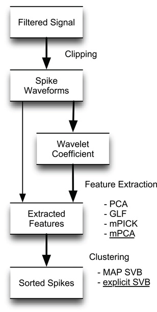
Figure 1. Overview of the various spike-sorting algorithms compared in this study. The algorithm proposed flows along thick arrows and consists of spike detection, feature extraction by mPCA in the space of wavelet coefficients, and spike sorting by explicit SVB.
Detection of Spike Candidates and Calculation of Spike Waveforms
Spike detection was performed as in the previous study (Takekawa et al., 2010). After high-pass filtering raw signals, spikes were detected by amplitude thresholding. The high-pass filter was designed to subtract Gaussian smoothed signals from the raw signals. The threshold was set to μrobust [h(t)]−fthr σrobust [h(t)], where h(t) is the high-pass filtered signal, fthr is the threshold factor and μrobust, σrobust are robust estimates of the average and the standard deviation, respectively (Hoaglin et al., 1983; Quian Quiroga et al., 2004; Takekawa et al., 2010).
For each detected spike candidate, we interpolated the discrete waveform around the peak with a quadratic spline and determined the precise spike timing as the peak of the interpolated line. A spike in general exhibits slightly different peak times at different channels. To avoid detecting the same spike more than once, the waveforms detected within a time window of 0.5 msec were regarded as the same spike. Then, we resampled the filtered signal at the same sampling rate as the filtered data in the range of discrete times [−τ1 :τ2] with applying a window function, where τ = 0 refers to the precise spike timing and a window function can be described as
where  is the normal distribution, and s = τ1 if τ < 0 or otherwise s = τ2. We will determine adequate values of these time constants later.
Feature Extraction
We applied mPCA with KS test for normality to the wavelet coefficients for feature extraction. The wavelet coefficients are calculated by multi-resolution analysis with Chohen-Daubechies-Feauveau 9/7 (CDF97) wavelet (Cohen et al., 1992; Daubechies, 1992; Takekawa et al., 2010). The multi-resolution analysis is analogous to discrete Fourier transform and transforms data in the time domain to those of time-frequency coefficients preserving the data dimension. To evaluate the performance of the method, we applied PCA, GLF, mPICK, and mPCA to the data set of resampled waveforms or the wavelet coefficients of the waveforms. Below we outline the frameworks of these feature extraction algorithms.
Principle component analysis
The algorithm of PCA is well described in literature and is only briefly reviewed (Bishop, 2006). The original D-dimensional data X = {xn}Nn = 1 is reduced to a D′-dimensional data through the linear transformation VT XC, where XC = {xn − E[x]}Nn = 1, and the projection matrix V is constructed from the eigenvectors corresponding to the largest D′ eigenvalues λ1 ≥ λ2 ≥ ··· ≥ λD′ of the covariance matrix of XC. The data points exhibit the largest D′ variances in thus obtained D′-dimensional subspace.
Graph laplacian features
Below, the definition and derivations of GLF are briefly reviewed. Details are found in (Ghanbari et al., 2011). As in the case of PCA, the original D-dimensional data set X = {xn}Nn = 1 is reduced to a D′-dimensional data set through the transformation Y = AT X, where A = {ad}D′d = 1 and ad is a D-dimensional vector. It is desirable in classification if neighboring points in the original D-dimensional space remain close to each other after a projection to the low dimensional space (He and Niyogi, 2004).
Such a projection A can be obtained by solving the following minimization problem:
where W is a weight matrix and Y = {yn}Nn = 1 is reduced data set. Data points i and j are connected by an edge if i is among the K-nearest neighbors of j, or vice versa. The weight of the edge connecting these points is set as Wij = exp(−|xi − xj|2/t). If the two points are not among the K-nearest neighbors of one another, Wij = 0. The scaling parameter t is defined as
where  is the most distant point amongst the K-nearest neighbors of xi. We used K = 5 in this paper.
It is possible to rewrite the minimization problem as the following eigenvalue problem (Ghanbari et al., 2011):
where  with B and Q being N × N matrices defined as,
The projection matrix A = {ad}D′d = 1 is constructed from the eigenvectors corresponding to the largest D′ eigenvalues λ1 ≥ λ2 ≥ ··· ≥ λD′ of the matrix B.
Multimodality pickup
If values of some components are distributed with multiple peaks, we may use these components to separate a large number of clusters in the data. In mPICK, we picked up the wavelet coefficients that distribute with multiple peaks by employing KS test for the normality (Press et al., 1992; Quian Quiroga et al., 2004), which evaluates the deviation of given distribution from the normal (unimodal) distribution. Namely, forgiven one-dimensional data set x, KS test uses the maximum value of the absolute difference between the cumulative distribution function CDF of the normalized data x′ and that of a standard normal distribution for the evaluation:
We select the components corresponding to D′ largest values of ML [x]. Note that we use the robust statistical estimation for the mean and variance of the normalized data in order to minimize the effect of outliers. When we use mPICK without WT, we apply KS test to the distribution of the values at each time point of all the detected spike waveforms and pick up the time points that yield large multimodality. It is noted that the redundancy can be generally large in the features extracted by mPICK.
Multimodality-weighted PCA
To reduce the redundancy, we scale data points in each component dimension so that the variance of the scaled data along the dimension may coincide with its multimodality. This scaling emphasizes the multimodality of the data distribution and dramatically increases the chance to detect components showing strong multimodality among components with large variances. We define the procedure of mPCA explicitly as follows. We scale the each component of data set as  (d = 1,…,D) using the multimodality ML [x] defined in previous section and XM is reduced to a D′-dimensional data through PT XM. The projection matrix P is constructed from the eigenvectors corresponding to the largest D′ eigenvalues λ1 ≥ λ2 ≥ ··· ≥ λD′ of the covariance matrix of XM.
Clustering with Variational Bayes for Student's t Mixture Model
The optimal number of components in a mixture model can be determined by several criteria including Akaike's information criteria (Akaike, 1974), Bayesian information criteria (Schwarz, 1978), minimum description length (Rissanen, 1978) or minimum message length (Wallace and Boulton, 1968; Agusta and Dowe, 2002). Then, for a given number of components, we may estimate the optimal values of model's parameters by the maximum likelihood method implemented by Expectation-Maximization (EM) algorithm (Dempster et al., 1977). Alternatively, Bayesian inference treats model's parameters as probabilistic variables and calculates their probability distributions (Bernardo and Smith, 1994). Furthermore, variational Bayes (VB) algorithms provide EM-like methods to calculate the lower bound of the model evidence, i.e., the free energy, for Gaussian-mixture models (Attias, 1999) and Student's t mixture models (Svensén and Bishop, 2005; Archambeau and Verleysen, 2007). VB for Student's t mixture models (SVB) exhibited an excellent model selection performance in spike sorting (Takekawa et al., 2010). Below, we outline the framework of our SVB method. The mathematical details of the SVB algorithm are found in Takekawa and Fukai (2009).
Statistical models and parameters
Student's t distributions have long tails compared with Gaussian distributions, and hence are used frequently for modeling data containing outliers. This is actually the case for spike sorting since multiunit recordings detect a number of noisy spikes from distant neurons. Student's t distribution  can be written in terms of normal
  and Gamma
  distributions as follows:
where x is a D-dimension data point. The parameters ν, μ, and S are the DOF parameter, the component mean vector and the component precision matrix, i.e., the inverse of the covariance matrix, respectively. Normal and Gamma distributions are defined in Section “Distributions.” Student's t distribution is thus a mixture of infinitely many normal distributions with the same mean. The scaling parameter u for the precision S depends on parameter ν through the gamma distribution, and a smaller value of ν corresponds to a heaver tail of  .
.
Our mixture model is described as a weighted sum of Student's t distributions:
where M is the number of clusters and θ = {αm,νm,μm, Sm}Mm = 1 represents the remaining model parameters. The weights αm are non-negative, and the parameters νm, μm, and Sm stand for the DOF, mean, and precision matrix of the m-th cluster, respectively. Introducing the latent label variables z = {zm}Mm = 1 and the latent scaling variables u = {um}Mm = 1, we can rewrite Student's t mixture model as a latent variable model:
The variable zm is unity if the data point belongs to the m-th cluster and is zero otherwise. Therefore, zm ∈ {0, 1} and only a single component of z can take a non-vanishing value. The variable um is necessary to analytically treat Student's t distribution in VB clustering. For a set of observations X = {xn}Nn = 1, the sets of variables Z = {zn}Nn = 1 and U = {un}Nn = 1 are called “latent variables”, where N represents the number of data points and the m-th component of zn (un), i.e., znm (unm), stands for zm (um) for the n-th data point. The latent variables are not direct observables but are inferred through a statistical model from other observed variables. The latent variables generally represent the degree to which variables move together. Hence, they play a crucial role in clustering of statistical data.
VB calculations for student's t mixture models
The VB is a general technique to solve for the posterior probability distribution of continuous variables. It calculates an approximate distribution of the posterior, assuming that the parameter variables and the latent variables are mutually independent. This assumption significantly reduces the cost of computations. Thus, in VB, we alternately renew the probability distributions of parameters and latent variables independently for a given prior distribution. In this study, we employ the factorized distributions for the priors as:
where,  and
and  represent Dirichlet, an exponential and a normal-Wishart distribution, respectively, with {κ0, ξ0, η0, γ0, μ0, Σ0} being the hyper parameters of the prior function (see Section “Distribution”).
Introducing a test distribution function qM (Z, U, θ) to approximate the posterior p(Z, U, θ|X, M) and assuming a factorization approximation qM(Z, U, θ) = qM (Z, U)qM(θ), we can describe the test function for model parameters qM(θ) and latent variables qM(Z, U) by hyper parameters  and
and  respectively:
where
And we can update these test functions by using an EM like iterative procedure.
In the M-step, the hyper parameters for model parameters  are updated using the data X and the current fixed hyper parameters for latent variables
where
and
In the E-step,  are updated using fixed
  obtained in the previous M-step.
where
Since the range of the integrations is from zero to infinity, on-demand calculations of the functional values of  and
and  at every step of the EM algorithm are quite time consuming. To avoid the heavy calculations, we may fix νm at the constant values estimated by MAP inference. Alternatively, here we explicitly treat νm as probabilistic variables and calculate the integrations by interpolating the values of
  and
and  from a numerical table calculated priori by Mathematica version 7 (Wolfram Research, Inc., Champaign, IL, 2008).
Model evidence and iterative algorithm
Using the ρnm calculated in the E-step, we can evaluate the model evidence as
The variable ρnm represents the likelihood that the n-th data point belongs to the m-th cluster. Therefore, the sum ∑Mm = 1 ρnm represents the degree to which the data point is described by the mixture model.
The reduced D'-dimensional data was decorrelated and renormalized before VB clustering so that μrobust and σrobust may be given as zero and unity, respectively. In order to reduce the effect of initial conditions, we preprocessed the data by k-means clustering (MacQueen, 1967) with sufficient large number of clusters and used the resultant clusters as initial conditions for VB clustering. Then we calculated E and M steps iteratively until (Fnew −Fold)/N <10−6 was satisfied and eliminate a cluster if its size or its variance was small or if it yielded a negative contribution to F. We can calculate the contribution to F of cluster m as
Many of the initial clusters were rapidly eliminated according to the criteria. Since most of the terms necessary for these evaluations appear in the calculations at E-step, no additional computational cost arises.
Each penalty term can be further calculated as


Distributions
The normal, Gamma, Dirichlet, exponential, Wishart and normal-Wishart distributions used in the text are defined as follows, respectively:
Data Set and Numerical Methods
We compared the performance of the proposed algorithm with that of other methods. To this end, we use a publicly available data sets of numerically simulated multiunit spike trains (Quian Quiroga et al., 2004; data sets are available at http://www2.le.ac.uk/departments/engineering/research/bioengineering/neuroengineering-lab/spike-sorting). The merit of this data base is that correct answers to spike sorting and the levels of difficulties are known for all the data sets. We employed the most difficult data sets, C_Easy2_noise20 [Ex2(0.20)], C_Difficult1_noise20 [Ex3(0.20)], and C_Difficult2_noise20 [Ex4(0.20)] in this study. All data sets contain spikes from three simulated neurons (see Figure 2). To obtain noisy signals, averaged spike waveforms with various amplitudes were added to each spike train at random times. In each data set, the standard deviation of noise was varied between 5 and 20% of the peak spike amplitudes. The simulated neural activity exhibits a firing rate of 20 Hz and a refractory period of 2 msec. The sampling rate of the all simulated data was assumed to 24 kHz.
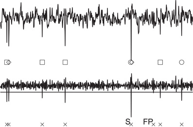
Figure 2. Simulated raw data [Ex4(0.20), upper] and high-pass filtered data (lower). The simulated raw data contains signals from three neurons, which are marked with circles, squares, and diamonds, respectively. The horizontal line shown for the filtered data is the threshold for spike detection, and crosses represent the detected spikes. The data contains a false negative spike (FP) and synchronized spikes that were detected as a single spike (S).
We also use the experimental data obtained by simultaneous extracellular and intracellular recordings (Harris et al., 2000; Henze et al., 2000; data sets are available at http://crcns.org/data-sets/hc/hc-1). In these data, the correct sequence of spikes is known at least for a single neuron recorded intracellularly, which implies that the correct answers to spike sorting are already partially known. We employed two different data sets, d11222.001 and d14521.001, in this study since an intracellularly recorded neuron exhibited burst firing in d11222.001 or it generated only 181 spikes during the whole period of recordings in d14521.001. The data sets were recorded at 20 kHz.
We implemented our spike sorting algorithms in C++ code with linear algebra routines in Lapack library (http://www.netlib.org/lapack/) and OpenMP parallelization (http://www.openmp.org/). The program was compiled by Intel Compiler with Lapack implementation of Math Kernel Library (Intel Corp.) and executed on Mac OS X environment (Mac Pro; 2 × 2.93 GHz Quad-Core Intel Xeon; Apple Inc.).
Results
The proposed method was tested on simulated and experimental data, and the results were compared with those of other methods.
Detection of Spike Candidates
In spike detection, we used fthr = 3 in thresholding for simulated data and fthr = 4 for simultaneous intracellular-extracellular recording data. Figure 2 shows examples of the spikes detected in the simulated data, in which spikes belonging to three different neurons are marked by different symbols. Note that the correct answers are known for the artificial spike data. Spikes from different neurons were sometimes detected as a single spike (synchronized spikes) if their temporal locations were close to each other (see S in Figure 2). While true spikes were rarely missed (i.e., almost no false negative), noisy signals were sometimes detected as spurious spikes (false positive: see FP in Figure 2).
Each simulated data contains spike trains of three neurons and noisy spikes, and we used the artificial spike data simulated at the highest noise level. Our method detected 3973 (Ex2), 3883 (Ex3), and 3916 (Ex4) candidate spikes in each artificial data set, while they should contain 3526, 3414, and 3493 correct spikes, respectively. The numbers of false positive, false negative, and synchronized spikes were 530, 6, and 77 (Ex2), 540, 0 and 72 (Ex3), and 496, 1 and 70 (Ex4), respectively, in these data sets. We obtained about 14,000 spike candidates in each data set of the simultaneous intracellular-extracellular recordings.
Feature Extraction
We applied PCA, GLF, mPICK, and mPCA to the three simulated data sets with or without the preprocessing by WT. Figure 3 shows the first two components of the extracted features. The range of parameters for clipping out the spike waveform was set as τ1 = 24 and τ2 =36. To see the degree of separation between spike clusters belonging to different neurons, we display the distribution of the features extracted by four different methods for each data set in Figure 3. Spikes belonging to three neurons and noisy clusters were labeled with different colors: spikes of the three neurons are shown in red, green, and blue, while false positive spikes and synchronized spikes are shown in gray and black, respectively. A visual inspection indicates that mPCA with WT ensures a high quality of separation compared with the other methods.
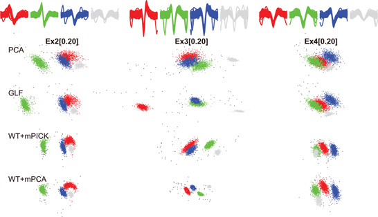
Figure 3. The features extracted from three data sets by PCA, GLF, WT + mPICK, and WT + mPCA. Red, blue, and green dots represent spikes belonging to three neurons. Gray dots stand for noisy spikes (false positives) and black dots for synchronized spikes. The clusters are shown in the two-dimensional feature space spanned by the first and second components. Top row shows the spike waveforms obtained for the individual clusters.
In order to quantify the quality of feature extraction, we calculated the smallest isolation distance and the largest Lratio (defined below) for the clusters corresponding to the three neurons. If cluster c contains Nc spikes, the isolation distance of the cluster is the Mahalanobis square distance value trΣ−1c (x−μc) (x−μc)T of the Nc-th closest noise spike x outside the cluster (Harris et al., 2001; Schmitzer-Torbert et al., 2005), where μc and Σc are the center and variance of the cluster, respectively. Thus, the isolation distance estimates the average distance expected between a spike cluster and an equally large ensemble of spikes existing outside of the cluster. Lratio measures the degree of noise contamination of a cluster and is calculated as
where CDFχ2 is the cumulative distribution function of the χ2 distribution. Noise spikes close to the center of the cluster contribute significantly to the above sum, while noise spikes far from the center contribute little. Thus, smaller Lratio implies a lower degree of noise contamination.
In Figure 4, we compared the performance of the different methods for feature extraction in the presence and absence of pre-processing by WT. To evaluate the robustness of each method against details of spike detection, we chose the clipping range of spike waveforms from all possible 16 combinations of the following values: τ1, τ2 ∈ {24, 36, 48, 60}. The dimension of the waveform data depends on the values chosen. For instance, if τ1 = τ2 = 24, the dimension is 24 + 24 + 1 (time origin) = 49. As in Figure 3, the dimension of the extracted features D′ was reduced to 2. Both isolation distance and Lratio indicate that only mPCA with WT exhibited an excellent performance robustly in all the cases tested. Other methods, for instance GLF and mPICK, are sensitive to the choice of the clipping parameters. Wavelet transform did not improve the results of PCA and GLF, while it significantly improved the results of mPICK and mPCA. For mPCA, the robust estimation of the mean and variance also significantly improved the performance and the robustness.
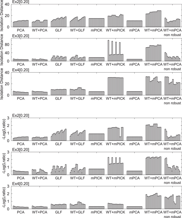
Figure 4. Minimum isolation distances and maximum L-ratios of the two-dimensional extracted features in three data sets. The worst cases (the minimum of the isolation distance and the maximum of the L-ratio) are shown for eight different methods: PCA, GLF, mPICK, and mPCA with or without the pre-processing by wavelet transform. In each method, results are shown for 16 different value sets of the two parameters for clipping out the spike waveform.
We evaluated the error rate in spike sorting also in a 3-dimensional feature space. Since the correct number of clusters is known to be four including a noise cluster, we employed a mixture of four Student's t distributions for spike clustering and the EM method for determining parameters of the model. The primary purpose here was to evaluate the best-expected performance of the different feature extraction methods. The total error ratio (false positive + false negative) was very large for the features extracted by PCA, WT + PCA, mPICK, and mPCA (Figure 5). By contrast, the error ratio was always very small for WT + mPCA compared with other methods. The robustness of the resultant clusters was degraded if the window function was not applied to spike waveforms (data not shown).
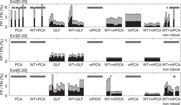
Figure 5. Evaluation of extracted features using optimal solution of clustering. Results are shown for eight different methods: PCA, GLF, mPICK, and mPCA with or without wavelet transform. Empty and filled bars represent the ratios of false negative and positive to the total spike number, respectively. The crosses in the diagrams mean that the bars do not fit into the chosen vertical limits.
Spike Clustering and Overall Sorting Quality on Physiological Data
Generally we need to repeat clustering of each data for different initial conditions to obtain stable results because of the conversion to local optima. However, we found that the error ratio and the free energy converged on almost identical values for different initial conditions if we used the initial condition calculated by k-means clustering (data not shown). Making an advantage of this robustness, we avoided the heavy averaging over initial conditions to significantly reduce the overall computational cost. We note that k-means clustering per se is much faster than VB clustering. However, whether our method produces accurate results without the averaging procedure should be examined with real physiology data. Below, we demonstrate this is actually the case.
In Figure 6, we applied MAP-SVB and explicit SVB to the features extracted from the spike data obtained by simultaneous intracellular-extracellular recordings. The clipping range of spike waveforms was varied across all possible combinations of τ1, τ2 ∈ {10, 15, 20, 25} and the dimension of the feature space was set equal to a realistic value of 12. The hyper parameters of prior distributions were set as κ0 =1 and η0 = 1, and μ0 and Σ0 were set as a zero vector and a unit matrix, respectively. Then, we investigated the effect of γ0 for MAP- and explicit SVB. Since γ0 represents a confidence factor of Σ0 in the Wishart distribution and Σ0 is a unit matrix, the variances of the estimated spike clusters become large for large values of γ0. This implies that the estimated number of clusters tends to be small for large γ0. On the contrary, spikes will be classified into many small clusters when γ0 is small. Accordingly, in the case of MAP-SVB a large γ0 value (γ0 = 60) yielded excellent results for bursting neurons (d11222.001), but it failed to give acceptable results for sparse-firing neurons (d14521.001). On the contrary, a small value (γ0 = 12) was suitable for sparse-firing neurons, but it did not work for bursting neurons. In fact for MAP-SVB, we could not find any intermediate value that ensures reasonably good results for both neuron types. In striking contrast, explicit SVB yields γ0 values that correctly separate the majority of spikes belonging to both neuron types in a wide range of the hyper-parameter value for the DOF parameter ν0 = 1/ξ0 (Figure 6). The noise level of experimental data was relatively small, and accordingly the difference in the performance between PCA and WT + mPCA was also small as compared with the case of artificial data. The results of WT + PCA and WT + GLF were similar to these of PCA and GLF, respectively, whereas the results of mPICK and mPCA were worse than those of WT + mPICK and WT + mPCA (data not shown).
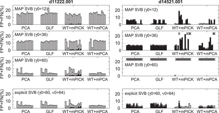
Figure 6. Error ratios in spike sorting in intra-extra data sets (d11222.001 and d14521.001). Empty and filled bars represent the ratios of false negative and positive to the total spike number, respectively. MAP-SVB cannot correctly classify both data at same hyper parameter value. On the other hand, explicit SVB can correctly classify both data with same setting of hyper parameter.
To explain why explicit SVB is advantageous over MAP-SVB, in Figure 7 we display the posterior distributions of the DOF parameters for the clusters estimated by the two methods. The DOF parameters estimated by MAP-SVB tend to distribute very broadly, implying that the estimated values may not be so reliable. Moreover, the values of the DOF parameters adopted in MAP-SVB, i.e., the values corresponding to the peak values of the posteriors, tend to be rather small. This results in very heavy tails in Student's t distributions of spike clusters. Therefore, MAP-SVB cannot always be a good method for estimating clustered distributions. In contrast, explicit SVB takes into account the shape of each posterior distribution in the cluster estimation and maintains the size of each distribution in a reasonably narrow range. This means that the confidence level for the estimation is expected to be high. Thus, the estimated clusters tend to show similar shapes and sizes without having extremely heavy tails.
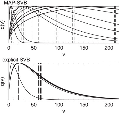
Figure 7. Typical examples of the posterior distributions of the DOF parameters for the clusters estimated by MAP-SVB and explicit SVB. For MAP-SVB, the vertical lines indicate the values that maximize the distributions. These values are used for the model estimation. For explicit SVB, the vertical lines indicate the average values of the distributions, and explicit SVB takes into account the shapes of the posterior distributions for the model estimation.
A major finding from the application of our method is that using mPCA on wavelet coefficients yields the most relevant features for clustering spikes by explicit SVB. Our results indicated that the KS test on wavelet coefficients is crucial for this improvement in feature extraction. We noticed that the method efficiently solves difficulties arising from outliers in the analysis of the multimodal distributions of wavelet coefficients (Figure 8A). Even a small amount of outliers affected the performance of the KS test if the conventional mean and variance are used (Figures 8B,C, left). Therefore, previous methods employed a special treatment to remove the influences of outliers in the KS test (Quian Quiroga et al., 2004). In contrast, the proposed KS test with the robust estimation of the mean and variance could evaluate various multimodal distributions with a surprising accuracy in the presence of outliers (Figures 8B,C right). More elaboration is necessary to clarify why the present KS test is so effective for the nature of spike signals. The wide repertoire of this KS test, which covers variety of multimodal distributions, may emerge partly from the inherent virtue of non-parametric estimation methods.
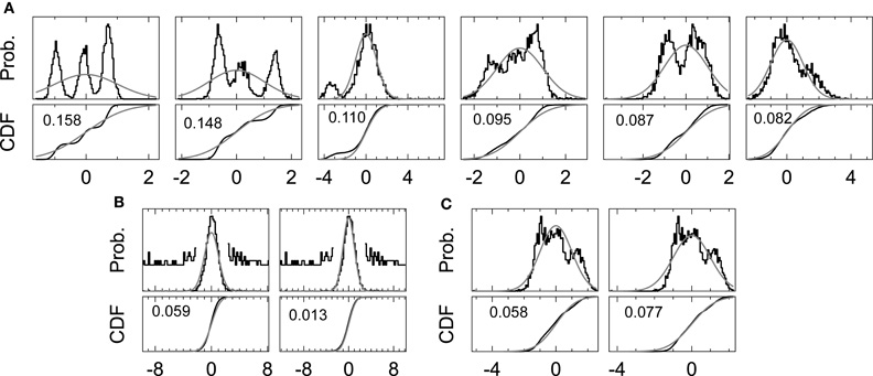
Figure 8. Comparison of the standard and proposed KS test on multimodality analysis.(A) The distributions of wavelet coefficients (upper) and the corresponding cumulative distributions (lower) are shown for the coefficients ranked in the top six of the multimodality ranking by the proposed KS test. In each panel, gray curve shows the Gaussian distribution compared with each multimodal distribution, and numbers indicate the values of the multimodality. (B, C) Unimodal and multimodal distributions with outliers were evaluated by the KS test with (right panel) and without (left panel) the robust estimation. Gray curves show the Gaussian distributions used in the evaluation. In B, the tails of the distributions are magnified by 20 to show outliers.
Computational Time
Computation time is another practically important measure in spike sorting. For simultaneous intracellular and extracellular recording data, the average computational cost of PCA, GLF, WT + mPICK, and WT + mPCA were about 2.4 s, 57.1 s, 2.1 s, and 2.9 s, respectively. The average computation time of explicit SVB was about 43.7 s. For comparison, the average computational cost was 46.0 s for a non-parallelized implementation of classification EM algorithms (KlustaKwik version 2.0.1 available at http://klustakwik.sourceforge.net).
Discussion
In order to improve the accuracy and speed of spike sorting, we have proposed a new algorithm based on mPCA and explicit SVB and compared the performance with several other spike-sorting methods on artificial and experimental spike data. We have demonstrated that the proposed method robustly yields the smallest error ratio to the total spike number among the methods tested. These improvements of the overall performance result from the multiple component mechanisms implemented in our method. First, the Gaussian window function applied to spike waveforms significantly improves the robustness and accuracy of the features extracted from spike waveforms. Second, mPCA enables us to extract informative features of spikes in a relatively low-dimensional feature space without sacrificing the computation speed of PCA. Third, the explicit numerical implementation of SVB significantly improves the robustness of clustering results, and the preprocessing by k-means clustering significantly reduces the overall computational cost of spike clustering by explicit SVB.
In particular, owing to explicit SVB our method successfully classified multi-neuron spikes even when the data contains spikes from both bursting neurons and sparse-firing neurons. Spike clustering of these neuron types was possible by several conventional methods if the spike data contains only one of these neuron types. However, when they coexist, we should initially introduce more clusters than actually needed so that we may manually combine the resultant spike clusters that likely belong to the same neurons. By this procedure, we may reduce the chance of the contamination of spikes from sparse-firing neurons. However, the manual inspection significantly decreases the efficacy of spike sorting, and possibly introduces human biases. Cortical neurons, especially those in the superficial cortical layers, fire very sparsely and some neurons in the deep cortical layer generate bursts of spikes. Therefore, explicit SVB employed by our method produces a significant practical merit.
The robustness of KS test is particularly important in mPCA as it weighs each feature dimension by the multimodality evaluated by the test. We may introduce some procedure, for instance the conventional normalization by the mean and variance, to suppress the influences of outliers on the evaluation of the normality. In practical spike sorting, however, we found that such a conventional method often did not work in the evaluation of the multimodality. In the present study, we have demonstrated that the robust estimation of the mean and variance enables us to correctly evaluate the multimodality and stabilizes the performance of mPCA. We have also tested other methods for mPCA based on SVB and Shannon's information criteria (Takekawa et al., 2010; Yang et al., 2010). However, none of these methods improved the accuracy of spike sorting compared with the present mPCA combined with KS test. In fact, they just created more parameters and heavier computational load.
Finally, the non-stationarity of extracellular recordings is another potential source of difficulty in spike sorting of real data. Drifts of recording electrodes or changes in the vital condition of cells may induce non-stationarity in the recorded signals. This problem has been addressed by several authors using different models (Pouzat et al., 2004; Bar-Hillel et al., 2006; Gasthaus et al., 2009). Recently, a clustering method that uses Kalman-filter mixture models for extracted features was proposed to overcome the difficulty (Calabrese and Paninski, 2011). Because the algorithm of VB for Kalman-filter mixture models is related to VB for linear Gaussian state-space models (Barber and Chiappa, 2007), we can in principle implement the method within the framework shown in this paper. However, since Kalman-filter mixture models require huge memory storage for large data sets, the method may not suit for sorting the spike data of long-term recordings. We examined the explicit SVB clustering method to obtain a computationally cheap method applicable to such data (data not shown), although the usability should be further validated.
Conflict of Interest Statement
The authors declare that the research was conducted in the absence of any commercial or financial relationships that could be construed as a potential conflict of interest.
Acknowledgments
This research was partially supported by KAKENHI 22700360, 23115524 (to Takashi Takekawa) and 22115013 (to Tomoki Fukai).
References
Abeles, M. (1982). Quantification, smoothing, and confidence limits for single-units' histograms. J. Neurosci. Methods 5, 317–325.
Agusta, Y., and Dowe, D. L. (2002). Clustering of Gaussian and t distribution using minimum message length,” in Proceedings of International Conference Knowledge Based Computer Systems (KBCS-2002). (Mumbai, India), 289–299.
Akaike, H. (1974). A new look at the statistical model identification. IEEE Trans. Automat. Contr. 19, 716–723.
Attias, H. (1999). “Learning parameters and structure of latent variables by variational Bayes,” in Proceeding of the 15th Conference on Uncertainty in Artificial Intelligence (Stockholm, Sweden), 21–30.
Barber, D., and Chiappa, S. (2007). “Unified inference for variational bayesian linear gaussian state-space models,” in Advances in Neural Information Processing Systems 19 (NIPS 2006). (Vancouver, Canada), 81–88.
Bar-Hillel, A., Spiro, A., and Stark, E. (2006). Spike sorting: Bayesian clustering of non-stationary data. J. Neurosci. Methods 157, 303–316.
Belkin, M., and Niyogi, P. (2003). Laplacian eigenmaps for dimensionality reduction and data representation. Neural Comput. 15, 1373–1396.
Brown, E. N., Kass, R. E., and Mitra, P. P. (2004). Multiple neural spike train data analysis: state-of-the-art and future challenges. Nat. Neurosci. 7, 456–461.
Calabrese, A., and Paninski, L. (2011). Kalman filter mixture model for spike sorting of non-stationary data. J. Neurosci. Methods 196, 159–169.
Câmara de Macedo, K. A., Scheiber, R., and Moreira, A. (2008). An autofocus approach for residual motion errors with applications to airborne repeat-pass SAR interferometry. IEEE Trans. Geosci. Remote Sens. 46, 3151–3162.
Chah, E., Hok, V., Della-Chiesa, A., Miller, J. J. H., O'Mara, S. M., and Reilly, R. B. (2011). Automated spike sorting algorithm based on laplacian eigenmaps and k-means clustering. J. Neural Eng. 8, 016006.
Cohen, A., Daubechies, I., and Feauveau, J. C. (1992). Biorthogonal bases of compactly supported wavelets. Comm. Pure Appl. Math. 45, 485–500.
Csicsvari, J., Hirase, H., Czurko, A., and Buzsáki, G. (1998). Reliability and state dependence of pyramidal cell-interneuron synapses in the hippocampus: an ensemble approach in the behaving rat. Neuron 21, 179–189.
Dempster, A. P., Laird, N. M., and Rubin, D. B. (1977). Maximum likelihood from incomplete data via the EM algorithm. J. R. Stat. Soc. Series B (Methodol.) 39, 1–38.
Fynh, M., Hafing, T., Treves, A., Moser, M. B., and Moser, E. I. (2007). Hippocampal remapping and grid realignment in enthorhinal cortex. Nature 466, 190–194.
Gasthaus, J., Wood, F., Gorur, D., and Teh, Y-W. (2009). “Dependent dirichlet process spike sorting,” in Advances in Neural Information Processing Systems 21 (NIPS 2008). (Vancouver, Canada), 497–504.
Ghanbari, Y., Papamichalis, P. E., and Spence, L. (2011). Graph-laplacian features for neural waveform classification. IEEE Trans. Biomed. Eng. 58, 1365–1372.
Halata, E., Rasmussen, C. E., Tolias, A. S., Sinz, F., and Logothetis, N. K. (2000). Detections and sorting of neural spikes using wavelet packets. Phys. Rev. Lett. 85, 4637–4640.
Harris, K. D., Henze, D. A., Cscicsvari, J., HIrase, H., and Buzsáki, G. (2000). Accuracy of tetrode spike separation as determined by simultaneous intracellular and extracellular measurments. J. Neurophysiol. 84, 401–414.
Harris, K. D., Hirase, H., Leinekugel, X., Henze, D. A., and Buzsáki, G. (2001). Temporal interaction between single spikes and complex spike bursts in hippocampal pyramidal cells. Neuron 32, 141–149.
He, X., and Niyogi, P. (2004). “Locality preserving projections,” in Advances in Neural Information Processing Systems 16 (NIPS 2003). (Whistler, Canada), 153–160.
Henze, D. A., Borhegyi, Z., Cscicsvari, J., Mamiya, A., Harris, K. D., and Buzsáki, G. (2000). Intracellular features predicted by extracellular recordings in the hippocampus in vivo. J. Neurophysiol. 84, 390–400.
Hoaglin, D. C., Mosteller, F., and Tukey, J. W. (1983). Understanding Robust and Exploratory Data Analysis. New York, NY: John Wiley & Sons Inc.
Lewicki, M. (1998). A review of methods for spike sorting: the detection and classification of neural action potentials. Network 9, R53–R78.
MacQueen, J. B. (1967). “Some methods for classification and analysis of multivariate observations,” in Proceedings of 5th Berkeley Symposium on Mathematical Statistics and Probability. (Berkeley, CA), 281–297.
O'Keefe, J., and Recce, M. L. (1993). Phase relationship between hippocampal place units and the EEG theta rhythm. Hippocampus 3, 317–330.
Pavlov, A., Makarov, V. A., Makarova, I., and Panetsos, F. (2007). Sorting of neural spikes: when wavelet based methods outperform principal component analysis. Neural Comput. 6, 269–281.
Pouzat, C., Delescluse, M., Viot, P., and Diebolt, J. (2004). Improved spike-sorting by modeling firing statistics and burst-dependent spike amplitude attenuation: a Markov chain Monte Carlo approach. J. Neurophysiol. 91, 2910–2928.
Press, W. H., Teukolsky, S. A., Vetterling, W. T., and Flannery, B. P. (1992). Numerical Recipes in C. Cambridge, MA: Cambridge University Press.
Quian Quiroga, R., Nadasdy, Z., and Ben-Shaul, Y. (2004). Unsupervised spike detection and sorting with wavelets and superparamagnetic clustering. Neural Comput. 16, 1661–1687.
Schmitzer-Torbert, N., Jackson, J., Henze, D., Harris, K. D., and RedishA. D. (2005). Quantitative measures of cluster quality for use in extracellular recordings. Neuroscience 131, 1–11
Svensén, M., and Bishop, C. M. (2005). Robust Bayesian mixture modeling. Neurocomputing 64, 235–252.
Takekawa, T., and Fukai, T. (2009). A novel view of the variational Bayesian clustering. Neurocomputing 72, 3366–3369.
Takekawa, T., Isomura, Y., and Fukai, T. (2010). Accurate spike sorting for multi-unit recordings. Eur. J. Neurosci. 31, 263–272.
Wallace, C. S., and Boulton, D. M. (1968). An information measure for classification. Comput. J. 11, 185–194.
Wilson, M. A., and McNaughton, B. L. (1993). Dynamics of the hippocampal ensemble code for space. Science 261, 1055–1058.
Wood, F., Fellows, M., Donoghue, J. P., and Black, M. J. (2004). “Automatic spike sorting for neural decoding,” in Proceedings of the 26th Annual International Conference of IEEE Engineering in Medicine and Biology Society (EMBC). (San Francisco, CA), 4009–4012.
Keywords: multiunit recording, classification, feature extraction, clustering, machine learning, wavelet transform, redundancy, robustness
Citation: Takekawa T, Isomura Y and Fukai T (2012) Spike sorting of heterogeneous neuron types by multimodality-weighted PCA and explicit robust variational Bayes. Front. Neuroinform. 6:5. doi: 10.3389/fninf.2012.00005
Received: 04 November 2011; Accepted: 01 March 2012;
Published online: 19 March 2012.
Edited by:
Marc-Oliver Gewaltig, Ecole Polytechnique Federale de Lausanne, SwitzerlandReviewed by:
Thomas Natschläger, Software Competence Center Hagenberg GmbH, AustriaXin Wang, The Salk Institute for Biological Studies, USA
Copyright: © 2012 Takekawa, Isomura and Fukai. This is an open-access article distributed under the terms of the Creative Commons Attribution Non Commercial License, which permits non-commercial use, distribution, and reproduction in other forums, provided the original authors and source are credited.
*Correspondence: Takashi Takekawa and Tomoki Fukai, RIKEN Brain Science Institute, Laboratory for Neural Circuit Theory, Hirosawa 2-1, Wako, Saitama, 351-0198, Japan. e-mail: takekawa@riken.jp; tfukai@riken.jp