Brian hears: online auditory processing using vectorization over channels
- 1 Laboratoire Psychologie de la Perception, CNRS and Université Paris Descartes, Paris, France
- 2 Département d’Etudes Cognitives, Ecole Normale Supérieure, Paris, France
The human cochlea includes about 3000 inner hair cells which filter sounds at frequencies between 20 Hz and 20 kHz. This massively parallel frequency analysis is reflected in models of auditory processing, which are often based on banks of filters. However, existing implementations do not exploit this parallelism. Here we propose algorithms to simulate these models by vectorizing computation over frequency channels, which are implemented in “Brian Hears,” a library for the spiking neural network simulator package “Brian.” This approach allows us to use high-level programming languages such as Python, because with vectorized operations, the computational cost of interpretation represents a small fraction of the total cost. This makes it possible to define and simulate complex models in a simple way, while all previous implementations were model-specific. In addition, we show that these algorithms can be naturally parallelized using graphics processing units, yielding substantial speed improvements. We demonstrate these algorithms with several state-of-the-art cochlear models, and show that they compare favorably with existing, less flexible, implementations.
1 Introduction
Models of auditory processing are used in a variety of contexts: in psychophysical studies, to design experiments (Gnansia et al., 2009) and interpret behavioral results (Meddis and O’Mard, 2006; Jepsen et al., 2008; Xia et al., 2010), in computational neuroscience, to understand the auditory system with neural modeling (Fontaine and Peremans, 2009; Goodman and Brette, 2010; Xia et al., 2010), in engineering applications, as a front end to machine hearing algorithms (Lyon, 2002; for example speech recognition, Mesgarani et al., 2006; or sound localization, May et al., 2011).
These models derive from physiological measurements in the basilar membrane (Recio et al., 1998) or in the auditory nerve (Carney et al., 1999), and/or from psychophysical measurements (e.g., detection of tones in noise maskers, Glasberg and Moore, 1990), and even though existing models share key ingredients, they differ in many details. The frequency analysis performed by the cochlea is often modeled by a bank of band pass filters (Patterson, 1994; Irino and Patterson, 2001; Lopez-Poveda and Meddis, 2001; Zilany and Bruce, 2006). While in simple models, filtering is essentially linear (e.g., gammatones, Patterson, 1994; or gammachirps, Irino and Patterson, 1997), a few models include non-linearities and feedback loops, such as the dynamic compressive gammachirp (DCGC; Irino and Patterson, 2001) and the dual resonance non-linear (DRNL) filter (Lopez-Poveda and Meddis, 2001), which are meant to reproduce non-linear effects such as level dependent bandwidth or two-tone suppression.
To simulate these models, many implementations have been developed, on software (O’Mard and Meddis, 2010; Patterson et al., 1995; Slaney, 1998; Bleeck et al., 2004), DSP board (Namiki et al., 2001), FPGA (Mishra and Hubbard, 2002), or VLSI (Watts et al., 1992) chips. But these implementations are all model-specific, which makes them difficult to use, modify, and extend according to the specific needs of the considered application. It also makes it difficult to compare different models. A second problem with current implementations of auditory models is that, due to memory constraints, they are often limited in the number of frequency channels they can work on simultaneously, typically tens or at most hundreds of channels, while there are about 3000 inner hair cells in a human cochlea.
To address the first problem, we designed a modular auditory modeling framework using a high-level language, Python. Python is a popular interpreted language with dynamic typing, which benefits from a variety of freely available libraries for scientific computing and visualization. This choice makes it easy to build complex auditory models, but it comes at the cost of a large interpretation overhead. To minimize this overhead, we used vectorization, an algorithmic strategy which consists in grouping identical operations operating on different data. This strategy was recently used to address similar issues in neural network simulation (Goodman and Brette, 2008, 2009).
By vectorizing over frequency channels, we can take advantage of the heavily parallel architecture of auditory models based on filter banks. In comparison, in available tools, model output is computed channel by channel. To avoid memory constraints with many channels, we use online processing. Finally, vectorization strategies are well adapted to parallelization on graphics processing units (GPUs), which follow the single instruction, multiple data (SIMD) model of parallel computing.
We start by describing our vectorization algorithms (see Section 2) before presenting their implementation in a modular auditory modeling toolbox (see Section 3). We illustrate the functionality and performance with “Brian Hears,”1 a Python toolbox developed by our group. Brian Hears is a library for the spiking neural network simulator package “Brian”2 (Goodman and Brette, 2008, 2009), which also relies on vectorization strategies (Brette and Goodman, 2011). To give an idea of how this tool facilitates auditory modeling and the integration with neural modeling, Figure 1 shows an auditory model consisting of a gammatone filterbank with half-wave rectification, compression, and spiking with integrate-and-fire models (but note that the toolbox can also be used independently of Brian). Finally, we compared the performance with existing implementations written in Matlab (Slaney, 1998; Bleeck et al., 2004), another high-level interpreted language.
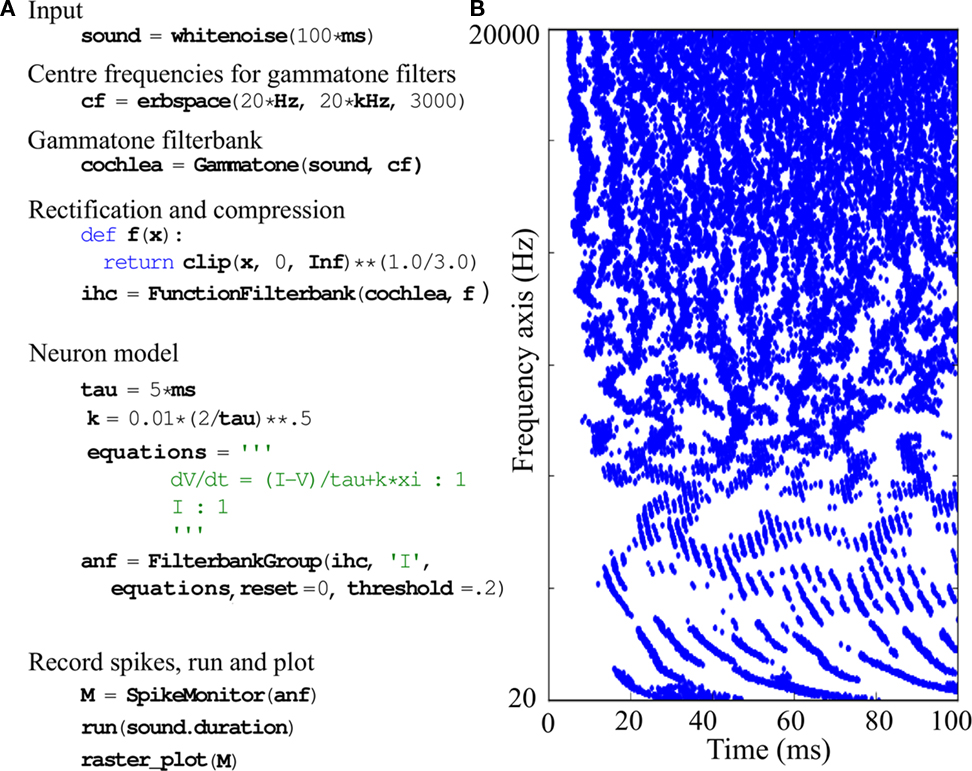
Figure 1. Simple spiking model of the auditory periphery. The cochlea and inner hair cells are modeled using gammatone filtering followed by half-wave rectification and 1/3-power law compression. We model the auditory nerve fibers as leaky integrate-and-fire neurons defined by the stochastic differential equation  where the current I is the output of the inner hair cell model and J(t) is physiological white noise (not the acoustic input noise). (A) Python implementation with the Brian Hears toolbox. Variable I in the neuron model is linked to the output of the filterbank. (B) Raster plot of the model output.
2 Algorithms
2.1 Vectorized Filtering Over Frequencies
Using a high-level interpreted language induces a fixed performance penalty per interpreted statement, which can add up to a significant cost if loops over large data sets are involved. Similar to Matlab, the NumPy (Oliphant, 2006) and SciPy (Jones et al., 2001) packages for Python address this problem for scientific computation. In order to add two large vectors x and y, we do not need to write for i in range(N): z[i] = x[i]+y[i] which would have an interpretation cost of O(N), but simply z = x+y with an interpretation cost of O(1).
Another problem that needs to be addressed is the very large memory requirements that standard implementations of auditory periphery models run into when using large numbers of channels. These implementations compute the entire filtered response to a signal for each frequency channel before doing further processing, an approach we call “offline computation.” For N channels and a signal of length M samples stored as floats, this means there is a memory requirement of at least 4 NM bytes which can quickly get out of hand. The human cochlea filters incoming signals into approximately 3000 channels. At a minimum sampling rate of 40 kHz this requires 457 MB/s to store, hitting the 4-GB limit of a 32-bit desktop computer after only 8.9 s (and even the larger amounts of memory available on 64 bit machines would be quickly exhausted).
We address both of these problems using “online computation” vectorized over frequencies. Specifically, at any time instant we store only the values of the filtered channels for that time instant (or for the few most recent time instants), almost entirely eliminating the memory constraints. This approach imposes the restriction that every step in the chain of our auditory model has to be computed “online” using only the few most recent sample values. For neural models, this is entirely unproblematic as filtered sample values will typically be fed as currents into a neural model consisting of a system of differential equations (see Figure 1). The restriction can, however, be problematic in the case of models which involve cross- or auto-correlation, although these can also be addressed by using online or buffered correlators.
As an example of vectorized filtering, consider a first order digital infinite impulse response (IIR) filter with direct form II transposed parameters a0 = 1, a1, b0, b1. For an input signal x(t) (with t an integer) the output signal y(t) can be computed by introducing an extra variable z(t) and using the difference equations:


By making x(t), y(t), and z(t) into vectors of length N for N frequency channels, this step can be coded as:
y = b[0]*x + z
z = b[1]*x − a[1]*y
For an order k IIR filter, this requires storage of 4 Nk bytes (for floats) or 8 Nk (for doubles), imposing low memory requirements even for very large numbers of channels or high order filters.
An additional benefit of vectorizing over frequency is that it allows us to make use of vectorized instruction sets in CPUs, or the use of highly parallel general purpose GPUs. Figure 2 shows the pseudocode for an IIR filterbank based on a direct form II transposed structure. The standard way to compute the response of a bank of filters in auditory modeling packages is Algorithm 1, that is doing the computation for each channel in order. However, Algorithm 2, in which the innermost loop is over channels, is able to make much more efficient usage of vectorized instruction sets. We consider implementations using Python, and C++ on CPU and GPU. In the Python implementation, the outer loop over samples is a Python loop and the innermost loops over channels and the filter order are vector operations using NumPy (which is coded in low-level C). In the GPU implementation, N threads are executed in parallel (for N the number of channels). Each thread loops over the number of samples and the filter order, so in effect the outer loops are performed explicitly and the inner loop is implicit in the fact that thread i operates on the data for channel i.
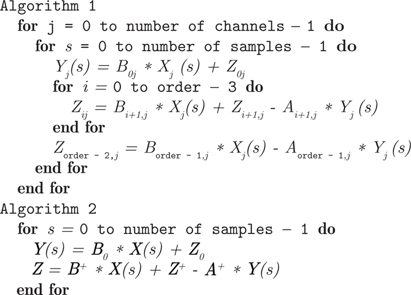
Figure 2. Pseudo code of the two algorithms for the direct form II transposed IIR filter, sequential channels (Algorithm 1) and vectorized channels and filter order (Algorithm 2). Bold faced variables are vectors of size the number of channels, subscripts j give elements of these vectors, and the * operation corresponds to element-wise multiplication. The input is X(s) and the output is Y(s), that is X j(s) is the sample in channel j at time s and similarly for Y(s). A i and B i are the parameters of the filter (which can be different for each channel), and the Z i are a set of internal variables. Written without indices, A,B,Z refer to two-dimensional arrays, and the operations over these 2D arrays vectorize over both channels and the order of the filter. The notation Z+ refers to a shift with respect to the filter order index, so that  The variable “order” is the order of the filter. For Algorithm 2, in Python, the code reads almost directly as above. In C++ on the CPU, it reads as above but each line with a vector operation has a loop. On the GPU it reads as above, but is evaluated in parallel with one thread per channel and a loop over the filter order.
In each case, certain optimizations can be performed because of the presence of the inner loop over channels. If we wish to compute the response of an IIR filter for a single frequency channel, we are required to compute the time steps in series, and so we cannot make use of vector operations such as the streaming SIMD extensions (SSE) instructions in x86 chips. Computing multiple channels simultaneously however, allows us to make use of these instructions. Current chips feature vector operations acting on 128-bit data (four floats or two doubles) with 256 or 512 bit operations planned for the future. In the C++ version, on modern CPUs Algorithm 2 performs around 1.5 times as fast as Algorithm 1 (see for instance Figures 7 and 8). GPUs allow for even better parallelism, with the latest GPUs capable of operating on 512 floats or doubles in parallel. In principle this would seem to allow for speed increases of up to 512 times, but unfortunately this is not possible in practice because computation time becomes memory bound and memory access speeds have not kept pace with the ability of GPUs to process data. Transfer from GPU global memory to thread local memory can often take hundreds of times longer than executing an instruction (although this can be alleviated using coalesced memory access). Even worse problems are caused if the data needs to be uploaded to the GPU, processed and then downloaded back to the CPU, due to the limited memory bandwidth. The results of these vectorization optimizations are shown in Section 3.5.
2.2 Buffering
Vectorizing over frequency is useful but also introduces some problems. Firstly, if we have a high sample rate then in an interpreted language we will have a high interpretation cost if we have to process loops each time step. For example, the Python pass operation (which does nothing) takes around 15ns to execute. If we have to do 100 Python operations per time step at a 40-kHz sampling rate, then the interpretation time alone would be at least 60 ms per second. The second problem with vectorizing over frequency is that it may be useful to store filtered values for a certain amount of time, for example to implement an online correlator with a short time constant, such as in the auditory image model (AIM; Patterson, 2000).
To address this, we can use a system of buffered segments. For a filter with N channels, we compute the response to K samples at a time, returning a 2D array with shape (K, N), where the parameter K can be varied. This has several computational consequences. First of all, we can reduce the number of interpreted instructions. In a chain of filters, the input of each filter is fetched via a function (or more precisely, method) call to the previous filter in the chain. In Python, function calls have a relatively large interpretation overhead and so in a chain of several filters this combined overhead can add up to a substantial amount if the functions were called every time step. However, if the chain of function calls only needs to be made once every K steps the corresponding overhead will be reduced by a factor of K. If we are using only Python and NumPy, we still have some Python instructions for each timestep but these are smaller than the overheads associated to the chain of function calls. We can reduce these overheads even more by implementing some special cases directly with C/C++ code. For example, many filters build on a cascade of IIR filters, and so by writing a Python extension for computing the buffered response of a bank of filters to such a cascade, we reduce the interpretation cost to once every K samples.
It turns out that for FIR filters of reasonable length, an FFT-based algorithm is usually much more efficient than a convolution, and a buffered system allows us to use this more efficient algorithm. Note that an FFT algorithm can also be vectorized across frequencies, although this comes at the cost of a larger intermediate memory requirement.
Combining vectorization over frequency and buffering allows us to implement an efficient and flexible system capable of dealing with large numbers of channels in a high-level language. There are several trade-offs that need to be borne in mind, however. First of all, large buffer sizes increase memory requirements. Fortunately, this is normally not a problem in practice, as smaller buffer sizes can actually improve speed through more efficient usage of the memory cache. Depending on the number of frequency channels and the complexity of the filtering, there will be an optimal buffer size, trading off the cache performance for smaller buffers against the increased interpretation cost. In our implementation, a buffer size of 32 samples gives reasonable performance over a fairly wide range of parameters, and this is the default value. For FFT-based FIR filtering, the tradeoff is different, however, because with an impulse response of length L and a buffer of length K we need to apply an FFT of length L + K. If K < L then most of this computation will be wasted. The default implementation uses a buffer size K = 3L for reasonable all-round performance (with the added benefit that if the impulse response length is a power of 2, L + K will also be a power of 2, for a more efficient FFT).
3 Implementation and Results
3.1 Modular Design
In order to make the system as modular and extensible as possible, we use an object-oriented design based on chains of filter banks with buffered segments as inputs and outputs. Since processing is vectorized over frequency channels, inputs, and outputs are matrices (the two dimensions being time and frequency). Figure 3A. shows an example of a complex cochlear model, the DRNL model (Lopez-Poveda and Meddis, 2001), which consists of the filtering of an input – stapes velocity – by a linear and a non-linear pathway. Each box in the diagram corresponds to a specific type of filterbank. The base class for these filterbanks defines an interface for passing buffered segments (as described in Section 2.2), allowing us to chain together multiple sound sources and filterbanks. There are default implementations of the general methods, for example to keep track of sample indices, cacheing previously computed values, and so forth. This means that to design a new filterbank class, one typically implements a single method that takes an input buffered segment and returns an output buffered segment. Three implementations can be used depending on available software and hardware. The basic implementation uses only Python and the NumPy package. If a suitable compiler is detected (gcc or Microsoft Visual C++), a C++ version will be used. Code is automatically generated and compiled behind the scenes (unrolling loops over the filter order if it is reasonably small). Finally, if an NVIDIA GPU is present, and the user has installed the PyCUDA package (Klöckner et al., 2009), filtering can be done on the GPU. At the moment, our GPU algorithms are essentially identical to the vectorized CPU algorithms, with no specific optimization. Although IIR filtering is fast on GPU, there is a bottleneck involved in transferring data to and from the GPU (see Section 2.1).
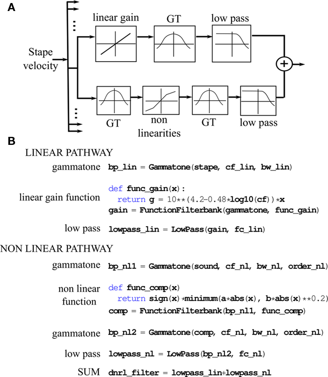
Figure 3. Dual resonance non-linear model of basilar membrane filtering. (A) Box representation of one frequency channel of the DRNL cochlear model. (B) Python implementation of the full model using the Brian Hears toolbox.
The example in Figure 3 shows two types of built-in filterbanks: IIR filterbanks and application of a static function. IIR filtering is implemented in a base class which uses a standard direct form II transposed structure, as discussed in Section 2.1. Several filterbanks derive from this class, for example gammatone and low-pass filters in Figure 3B. Other linear filterbanks are included, such as gammachirp and Butterworth filterbanks. Realistic models of cochlear processing also include non-linearities. In general, these are modeled as static non-linearities, that is, a given function is applied to all sample values across time and frequency. For example, in Figure 1, all channels are half-wave rectified (the NumPy function clip(input, 0, Inf) returns the values in the array input clipped between 0 and infinity) and compressed with a 1/3-power law (** is the exponentiation operator in Python). Another compressive function is applied in the DRNL model shown in Figure 3B. FIR filtering is also implemented, and uses an FFT-based algorithm, as discussed in Section 2.2.
3.2 Online Computation
As discussed in Section 2, in order to work with large numbers of channels we can only store a relatively small number of samples in memory at a given time. Traditionally, auditory models compute the entire output of each channel one by one, and then work with that output. This allows for very straightforward programming, but restricts the number of channels or lengths of sounds available. By contrast, working with buffered segments which are discarded when the next buffered segment is computed requires slightly more complicated programming, but not substantially. To compute a value that is defined over the entire signals (for example the power), one needs to calculate this quantity for each buffered segment in turn and combine it with the previous quantity. This corresponds to the “reduce” or “fold” algorithms in functional languages (reduce in Python), where an operator (e.g., addition) is applied to a list. For example, suppose we wanted to compute the RMS value of the outputs of all of the channels, we would keep a running total of the sum of the squared values of the outputs and then at the end divide by the number of samples and take the square root. This can be achieved using the filterbank process method as follows:
def sumsquares(input, running):

      return running+sum(input**2, axis=0)

ss = fb.process(sumsquares)

rms = sqrt(ss/nsamples)
The function sumsquares takes two arguments input (a buffered segment of shape (bufsize, nchannels)) and running. The second argument is initially 0, and then for each subsequent call will be the value returned by the previous call. The process method takes as argument a function which is assumed to have two arguments of the form above, and returns the final value returned by the function. In the example above, the sumsquares function keeps a running total of the sum of the squared values output by the filterbank. At the end of the computation, we divide by the number of samples to get the mean squared value, and then take the square root. The final value is an array of length nchannels. This mechanism allows us to do many online computations very straightforwardly. For more complicated online computations, users need to write their own class derived from the base filterbank class. This is also straightforward, but we do not show an example here.
3.3 Feedback
Some auditory models include feedback, e.g., in (Irino and Patterson, 2001; Zilany and Bruce, 2006), where filter parameters such as center frequency in the signal pathway is changed in response to the output of the control pathway (to perform adaptive gain control or bandwidth level dependence, for example). In Brian Hears this can be achieved using a feedback control filterbank. The user specifies an update function which takes one or several input filterbanks as arguments, and modifies the parameters of a target filterbank. This update function is called at regular intervals, i.e., every m samples. This is illustrated in Figure 4: a sound is passed through a control pathway – here a simple low-pass filter – and through a signal pathway – here a bandpass filter. The center frequency of the bandpass filter is controlled by the output of the control path.
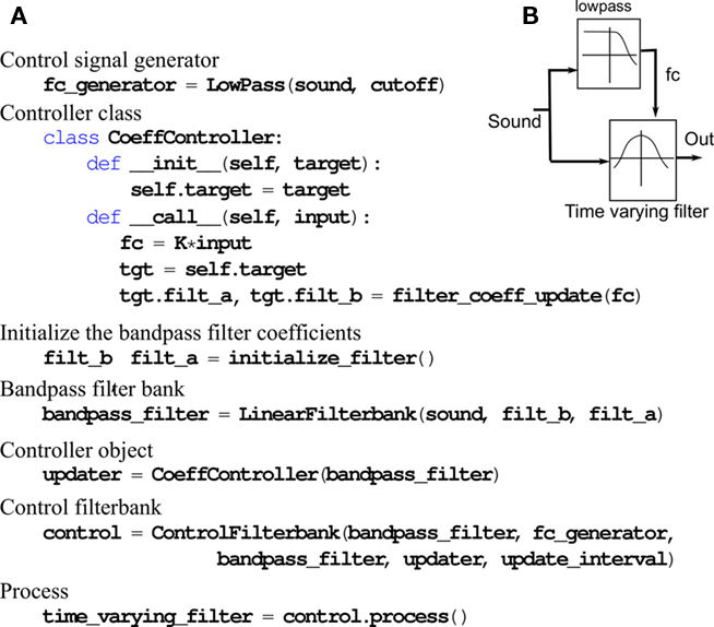
Figure 4. Auditory model with feedback. (A) Python program defining a time-varying filterbank with center frequency modulated by the output of a low-pass filter using the Brian Hears toolbox. (B) Corresponding box representation.
Updating the filter coefficients at every sample is computationally expensive and prevents us from using buffers. A simple way of speeding up the computation is to update the time-varying filter at a larger time interval. In Figure 5, we plotted the computation time against the update interval for the DCGC model (Irino and Patterson, 2001), using a 1.5-s sound with high dynamic range from the Pittsburgh Natural Sounds database (Smith and Lewicki, 2006). When the update interval is increased by just a few samples, the computation time is dramatically reduced. For longer intervals (above about 15 samples), the computation time reaches a plateau, when the feedback represents a negligible proportion of the total computation time. However, increasing the interval introduces errors, especially if the dynamic range of the sound is high. To analyze this effect, we processed the same dynamic sound at three different intensities between 30 and 90 dB SPL. The error-to-signal ratio (ESR) in dB is calculated between the output of the DCGC with an update interval of 1 sample (minimum error) and an update interval of i samples as follows:
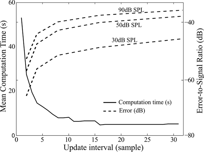
Figure 5. Performance of the dynamic compressive gammachirp model (DCGC) as a function of update interval. Solid line, left axis: computation time; Dashed lines, right axis: error-to-signal ratio for sounds at three different levels (30, 50, and 90 dB).

where RMS stands for root mean square and S(i) is the 2-dimensional output of the DCGC with an update interval of i samples. For very large time intervals, the error converges to the difference between the linear and non-linear filterbank, i.e., a time-varying and constant filterbank: −38 dB when the signal is at 30 dB SPL, −24 dB at 50 dB SPL, and −10 dB at 90 dB SPL. The effect of non-linearities is strongest at high input levels: at 90 dB SPL, the additional contribution of non-linearities to the signal has amplitude −10 dB compared to the signal obtained without non-linearities. As a comparison, when the feedback interval is about 15 samples (so that the feedback mechanism does not slow down computations), the error made by the algorithm at this level is about −38 dB. This means that the non-linear contribution is estimated with precision −28 dB, that is, about 4%. This seems reasonably accurate, especially given that simulation speed is almost not impacted by the feedback.
3.4 Vectorization Over Multiple Inputs
The benefits of vectorization are greatest when many channels are synchronously processed. This strategy extends to the simultaneous processing of multiple inputs. For example, consider a model with stereo inputs followed by cochlear filtering. Instead of separately processing each input, we can combine the cochlear filtering for the two mono inputs into a single chain, either in series, i.e., L1 L2…LNR1R2…RN or interleaved, i.e.,L1 R1 L2 R2…LNRN. Additionally, inputs can be repeated (ABC → AAABBBCCC) or tiled (ABC → ABCABCABC). We give an example in Figure 6, derived from a recent sound localization model (Goodman and Brette, 2010). Before reaching the inner ear the sound is filtered by the head related transfer function (HRTF). Each source location corresponds to a specific pair of HRTFs (left and right ear). The two filtered sounds at each ear are then decomposed into frequency bands by the basilar membrane, modeled as a gammatone filterbank (with up to 200 channels in (Goodman and Brette, 2010)), and further processed by neuron models (not shown in the Figure). The effect of sound location on neural responses can be simultaneously processed by vectorizing over channels and sound locations (i.e., over the whole set of HRTF pairs).
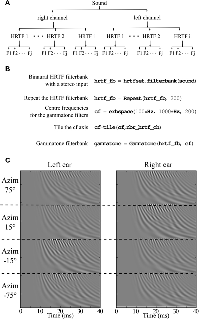
Figure 6. Vectorization over frequency and multiple head related transfer functions (HRTFs). (A) Schematic of nested vectorization over multiple HRTFs and frequencies. (B) Corresponding Python code. (C) Stereo output of the filterbank for four HRTF pairs.
3.5 Performance
We evaluated the performance of our algorithms for two models: a gammatone filterbank (Figure 7) and a DRNL filterbank (Figure 8). We compared them with non-vectorized implementations taken from existing toolboxes: Slaney’s Matlab toolbox for the gammatone filterbank (Slaney, 1998), and Meddis’s Matlab toolbox for the DRNL (Meddis, 2010), which we improved with respect to memory allocation to allow a fair comparison. In these implementations, frequency channels are processed in series using built-in filtering operations on time-indexed arrays (so that the interpretation cost is incurred once per frequency channel).
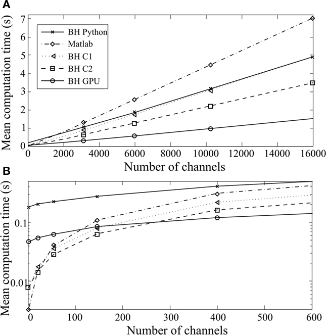
Figure 7. Computation time taken to simulate a gammatone filterbank as a function of the number of channels, with a 200-ms sound at 20 kHz [(B) is a magnified version of (A)]. Five different implementations are compared: Brian Hears in pure Python with vectorization over channels (BH Python), Brian Hears with C code generation, sequential channels (BH C1) or vectorized channels (BH C2), Brian Hears with GPU code generation, and Matlab with operations on time-indexed arrays.
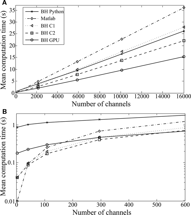
Figure 8. Computation time taken to simulate a DRNL filterbank as a function of the number of channels, with the same algorithms as in Figure 6 [(B) is a magnified version of (A)].
Inputs were 200-ms sounds sampled at 20 kHz. We could not use longer sounds with the Matlab implementations, because of the memory constraints of these algorithms.
Similar patterns are seen for the two models. For many frequency channels, computation time scales linearly with the number of channels, and all our implementations perform better than the original ones in Matlab. The best results are obtained with the GPU implementation (up to five times faster). With fewer channels (Figures 7B and 8B), a larger proportion of computation time is spent in interpretation in Python (BH Python), which makes this implementation less efficient. However, when low-level vectorized filtering is implemented in C (BH C2, vectorized channels), interpretation overheads are reduced and this implementation is faster than all other ones (except GPU) for any number of channels.
4 Discussion
To facilitate the use and development of auditory models, we have designed a modular toolbox, “Brian Hears,” written in Python, a dynamically typed high-level language.
Our motivation was to develop a flexible and simple tool, without compromising simulation speed. This tool relies on vectorization algorithms to minimize the cost of interpretation, making it both flexible and efficient. We proposed several implementations of vector-based operations: with standard Python libraries, C code, and GPU code. For models with many channels, all three implementations were more efficient than existing implementations in Matlab, which use built-in filtering operations on time-indexed arrays.
The GPU implementation was up to five times faster. With fewer channels, the best results were obtained with vectorization over channels in C.
The online processing strategy allows us to simulate models with many channels for long durations without memory constraints, which is not possible with other tools relying on channel by channel processing. This is important in neural modeling of the auditory system: for example, a recent sound localization model based on selective synchrony requires many parallel channels (Macdonald, 2008). In addition, online processing is required for a number of physiological models with feedback (Irino and Patterson, 2001; Lopez-Poveda and Meddis, 2001). The tool we have developed can be used to simulate and modify all these models in a simple way, with an efficient implementation and a direct interface to neuron models written with the Brian simulator. Figure 9 illustrates this possibility with the example of the stereausis model, an influential sound localization model (Shamma, 1989) which relies on correlations between overlapping frequency channels. In this model, the interaural time difference (ITD) sensitivity of binaural neurons is explained by the traveling wave velocity along the cochlea, i.e., higher frequencies arrive earlier than lower frequencies (Figure 9A). In the implementation with spiking neurons shown in Figure 9B, each pair of ipsilateral and contralateral fibers is connected to a specific coincidence detector, modeled as an integrate-and-fire neuron. Each binaural neuron fires if its inputs arrive at the same time. Therefore, if the inputs at both ears are identical (Figure 9C), i.e., the sound source lies on the median plane (ITD = 0 ms), the neurons on the diagonal will fire (ckk is the spike count of these neurons). If there is a delay between the ipsilateral and contralateral inputs (Figure 9D), i.e., if the source is not at the center, neurons above or under the main diagonal will fire. Thus the ITD of the sound source is represented by the activation of coincidence detectors. Using Brian Hears, the code for this model can be written in about a dozen lines (Figure 9B).
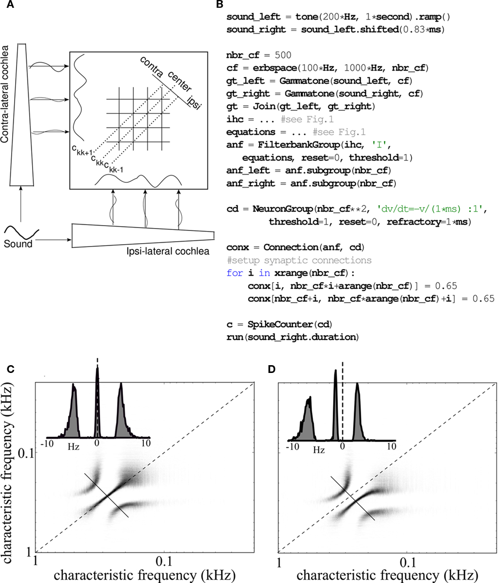
Figure 9. Stereausis model of sound localization. (A) Schematic of the stereausis binaural network. Ipsilateral and contralateral auditory nerve fibers project to coincidence detectors (each pair of fibers projects to a specific neuron). (B) Python implementation with the Brian Hears toolbox. (C) Spike counts of all coincidence detectors (horizontal: characteristic frequency (CF) of the ipsilateral input, vertical: CF of the contralateral input) in response to a 500-ms tone at 200 Hz presented simultaneously at both ears. The inset shows spike counts along the short diagonal line, as a function of CF difference between the two inputs. (D) Same as (C) but with the tone shifted by 830 μs at the contralateral ear.
Currently, the Brian Hears library includes: stimulus generation (e.g., tone, white, and colored noise) and manipulation (e.g., mixing, sequencing), including binaural stimuli, various types of filterbanks (e.g., gammatone, gammachirp, standard low-pass and bass filters, FIR filters), feedback control, static non-linearities, and a few example complex cochlear models. It also includes spatialization algorithms, to generate realistic inputs produced by sound sources in complex acoustical environments. These use similar vectorization techniques, and include models of reflections on natural surfaces such as grass or snow (Komatsu, 2008), the image method for reflections in square rooms (Allen and Berkley, 1979), and a raytracing algorithm to render any acoustical scene and produce realistic binaural stimuli, in combination with HRTF filtering. We believe this library will be useful for the development of auditory models, especially those including neural models. It should also be useful to design psychophysical experiments, as there are many Python packages for designing graphical user interfaces.
As we have shown, vectorized algorithms are well adapted to GPUs, which are made of hundreds of processors. In this work, we ported these algorithms to GPUs with no specific optimization, and it seems likely that there is room for improvement. Specifically, in the current version, all communications between different components of the models go through the CPU. This choice was made for simplicity of the implementation, but it results in unnecessary memory transfers between GPU and CPU. It would be much more efficient to transfer only the output spikes from the GPU to the CPU. We believe the most promising extension of this work is thus to develop more specific algorithms that take advantage of the massive parallel architecture of these devices.
Conflict of Interest Statement
The authors declare that the research was conducted in the absence of any commercial or financial relationships that could be construed as a potential conflict of interest.
Acknowledgments
This work was supported by the European Research Council (ERC StG 240132).
Footnotes
References
Allen, J. B., and Berkley, D. A. (1979). Image method for efficiently simulating small-room acoustics. J. Acoust. Soc. Am. 65, 943–950.
Bleeck, S., Ives, T., and Patterson, R. D. (2004). Aim-mat: the auditory image model in matlab. Acta Acoustica 90, 781–787.
Brette, R., and Goodman, D. F. M. (2011). Vectorised algorithms for spiking neural network simulation. Neural Comput. 23, 1503–1535.
Carney, L. H., McDuffy, M. J., and Shekhter, I. (1999). Frequency glides in the impulse responses of auditory-nerve fibers. J. Acoust. Soc. Am. 105, 2384–2391.
Fontaine, B., and Peremans, H. (2009). Bat echolocation processing using first-spike latency coding. Neural Netw. 22, 1372–1382.
Glasberg, B. R., and Moore, B. C. J. (1990). Derivation of auditory filter shapes from notched-noise data. Hear. Res. 47, 103–138.
Gnansia, D., Péan, V., Meyer, B., and Lorenzi, C. (2009). Effects of spectral smearing and temporal fine structure degradation on speech masking release. J. Acoust. Soc. Am. 125, 4023–4033.
Goodman, D. F. M., and Brette, R. (2008). Brian: a simulator for spiking neural networks in Python. Front. Neuroinformatics 2:5.
Goodman, D. F. M., and Brette, R. (2010). Spike-timing-based computation in sound localization. PLoS Comput. Biol. 6, e1000993.
Irino, T., and Patterson, R. D. (1997). A time-domain, level-dependent auditory filter: the gammachirp. J. Acoust. Soc. Am. 101, 412–419.
Irino, T., and Patterson, R. D. (2001). A compressive gammachirp auditory filter for both physiological and psychophysical data. J. Acoust. Soc. Am. 109, 2008–2022.
Jepsen, M. L., Ewert, S. D., and Dau, T. (2008). A computational model of human auditory signal processing and perception. J. Acoust. Soc. Am. 124, 422–438.
Jones, E., Oliphant, T., Peterson, P., et al. (2001). SciPy: Open Source Scientific Tools for Python. Available at: http://www.scipy.org/
Klöckner, A., Pinto, N., Lee, Y., Catanzaro, B., Ivanov, P., and Fasih, A. (2009). PyCUDA: GPU run-time code generation for high-performance computing. Available at: http://arxiv.org/abs/0911.3456
Komatsu, T. (2008). Improvement of the Delany–Bazley and Miki models for fibrous sound-absorbing materials. Acoust. Sci. Technol. 29, 121.
Lopez-Poveda, E. A., and Meddis, R. (2001). A human nonlinear cochlear filterbank. J. Acoust. Soc. Am. 110, 3107–3118.
Macdonald, J. A. (2008). A localization algorithm based on head-related transfer functions. J. Acoust. Soc. Am. 123, 4290–4296.
May, T., van de Par, S., and Kohlrausch, A. (2011). A probabilistic model for robust localization based on a binaural auditory front-end. IEEE Trans. Audio Speech Lang. Process. 9, 1–13.
Meddis, R. (2010). Auditory Modelling. Available at: http://www.essex.ac.uk/psychology/psy/PEOPLE/meddis/webFolder10/WebIntro.htm
Meddis, R., and O’Mard, L. P. (2006). Virtual pitch in a computational physiological model. J. Acoust. Soc. Am. 120, 3861–3896.
Mesgarani, N., Slaney, M., and Shamma, S. A. (2006). Discrimination of speech from nonspeech based on multiscale spectro-temporal modulations. IEEE Trans. Audio Speech Lang. Process. 14, 920–930.
Mishra, A., and Hubbard, A. E. (2002). A cochlear filter implemented with a field-programmable gate array. IEEE Trans. Circuits Syst. II 49, 54–60.
Namiki, M., Hamamoto, T., and Hangai, S. (2001). “Spoken word recognition with digital cochlea using 32 dsp-boards,” in Proceedings of the IEEE International Conference on Acoustics, Speech, and Signal Processing, Vol. 2 (Washington, DC: IEEE Computer Society), 969–972.
Oliphant, E. (2006). Guide to Numpy. Available at: http://www.tramy.us/
O’Mard, L. P., and Meddis, R. (2010). DSAM: Development System for Auditory Modelling. Available at: http://dsam.org.uk/
Patterson, R. D. (1994). The sound of a sinusoid: spectral models. J. Acoust. Soc. Am. 96, 1409–1418.
Patterson, R. D. (2000). Auditory images: how complex sounds are represented in the auditory system. J. Acoust. Soc. Jpn (E) 21, 183–190.
Patterson, R. D., Allerhand, M., and Giguere, C. (1995). Time-domain modelling of peripheral auditory processing: a modular architecture and a software platform. J. Acoust. Soc. Am. 98, 1890–1894.
Recio, A., Rich, N. C., Narayan, S. S., and Ruggero, M. A. (1998). Basilar-membrane responses to clicks at the base of the chinchilla cochlea. J. Acoust. Soc. Am. 103, 1972–1989.
Shamma, S. (1989). Stereausis: binaural processing without neural delays. J. Acoust. Soc. Am. 86, 989–1006.
Slaney, M. (1998). Auditory Toolbox: A Matlab Toolbox for Auditory Modeling Work. Technical Report 45, Apple Computer.
Watts, L., Kerns, D. A., Lyon, R. F., and Mead, C. A. (1992). Improved implementation of the silicon cochlea. IEEE J. Solid-State Circuits 27, 692–700.
Xia, X. J., Brughera, A., Colburn, H. S., and Shinn-Cunningham, B. (2010). Physiological and psychophysical modeling of the precedence effect. J. Assoc. Res. Otolaryngol. 11, 495–513.
Keywords: auditory filter, vectorization, Python, Brian, GPU
Citation: Fontaine B, Goodman DFM, Benichoux V and Brette R (2011) Brian hears: online auditory processing using vectorization over channels. Front. Neuroinform. 5:9. doi: 10.3389/fninf.2011.00009
Received: 19 May 2011;
Paper pending published: 05 June 2011;
Accepted: 30 June 2011;
Published online: 22 July 2011.
Edited by:
Daniel Gardner, Weill Cornell Medical College, USAReviewed by:
Ferenc Mechler, Medical College of Cornell University, USAWerner Van Geit, Okinawa Institute of Science and Technology, Japan
Copyright: © 2011 Fontaine, Goodman, Benichoux and Brette. This is an open-access article subject to a non-exclusive license between the authors and Frontiers Media SA, which permits use, distribution and reproduction in other forums, provided the original authors and source are credited and other Frontiers conditions are complied with.
*Correspondence: Romain Brette, Département d’Etudes Cognitives, Ecole Normale Supérieure, 29, rue d’Ulm, 75230 Paris, Cedex 05, France. e-mail: romain.brette@ens.fr