Does time ever fly or slow down? The difficult interpretation of psychophysical data on time perception
 Miguel A. García-Pérez
- Departamento de Metodología, Facultad de Psicología, Universidad Complutense, Madrid, Spain
Time perception is studied with subjective or semi-objective psychophysical methods. With subjective methods, observers provide quantitative estimates of duration and data depict the psychophysical function relating subjective duration to objective duration. With semi-objective methods, observers provide categorical or comparative judgments of duration and data depict the psychometric function relating the probability of a certain judgment to objective duration. Both approaches are used to study whether subjective and objective time run at the same pace or whether time flies or slows down under certain conditions. We analyze theoretical aspects affecting the interpretation of data gathered with the most widely used semi-objective methods, including single-presentation and paired-comparison methods. For this purpose, a formal model of psychophysical performance is used in which subjective duration is represented via a psychophysical function and the scalar property. This provides the timing component of the model, which is invariant across methods. A decisional component that varies across methods reflects how observers use subjective durations to make judgments and give the responses requested under each method. Application of the model shows that psychometric functions in single-presentation methods are uninterpretable because the various influences on observed performance are inextricably confounded in the data. In contrast, data gathered with paired-comparison methods permit separating out those influences. Prevalent approaches to fitting psychometric functions to data are also discussed and shown to be inconsistent with widely accepted principles of time perception, implicitly assuming instead that subjective time equals objective time and that observed differences across conditions do not reflect differences in perceived duration but criterion shifts. These analyses prompt evidence-based recommendations for best methodological practice in studies on time perception.
“There is nothing so practical as a good theory”
Lewin (1951, p. 169)
“There is nothing so theoretical as a good method”
Introduction
Time is crucial in our lives. We do not have a sense organ for time, but even infants 3–4 months old show some ability to discriminate short durations of different lengths (Provasi et al., 2011; Gava et al., 2012). During childhood and adolescence we develop a fine-grained perception of time surely based on our daily experience with objective time. Finely-tuned time perception seems to arise after higher-level cognitive processes are sufficiently developed (Block et al., 1999; Droit-Volet, 2013) and given explicit experience with objective time. It is nevertheless unclear whether our ability to represent and quantify time stems from a timing mechanism (an “internal clock”) that keeps track of time and can be read like a watch or, rather, only reflects our learning to translate experienced intervals into magnitudes expressed in the physical units of time that we got accustomed to. In the former case, empirical differences between subjective and objective time would be caused by an acceleration or deceleration of the internal clock, which thus gives an inexact reading (i.e., the internal clock is fast or slow); in the latter, they would reflect a subjective lengthening or shortening of duration, which nevertheless gets properly quantified afterwards. Figuring out which of these processes is taking place seems impossible because the process is unobservable and any observable outcome is compatible with these two and maybe also other accounts (Block, 1990; Grondin, 2010). Mechanistic accounts of timing processes have the status of metaphors (Wackermann, 2011), but difficulties to unravel those processes does not reduce our interest in investigating the phenomenon of time perception and the factors that affect it.
Time perception studies range from descriptions of the limits of our ability to judge and discriminate elapsed time or time differences, through the study of subject variables or stimulus conditions that affect such judgments, to assessments of distorted time perception in patients with psychiatric or neurological disorders. Detailed reviews have been published that describe the state and outcomes of this research in several areas (e.g., Grondin, 2010; Spence and Parise, 2010; Vroomen and Keetels, 2010; Allman and Meck, 2012; Chen and Vroomen, 2013; Allman et al., 2014) and this paper will not provide yet another review of this type. Our focus is instead on the methods used to gather data on the relation between subjective and objective time and on the conflicting or puzzling results that use of alternative (and presumably interchangeable) methods sometimes provides. Our main goal is to analyze the assumptions underlying these methods and to derive implications on the interpretation of data gathered with them. For this purpose, widely accepted principles of time perception will be built into a model of performance in psychophysical tasks in order to analyze the underpinnings, implications, and shortcomings of the various methods. To define our context, section Experimental Methods Used in Studies on Time Perception gives a brief overview of the classes of subjective and semi-objective methods used in studies on time perception. Section A Unified Model of Performance across Semi-Objective Psychophysical Tasks presents a model of performance in semi-objective psychophysical tasks that includes widely accepted components. Application of the model to different tasks in sections Single-Presentation Methods and Paired-Comparison Methods reveals how they can render conflicting results when time perception as implemented in the model is invariant across tasks. These results and their implications for best research practices are discussed in section General Discussion and Evidence-Based Recommendations.
Experimental Methods used in Studies on Time Perception
Research on time perception comprises two major types of study (Grondin, 2010): retrospective and prospective. Retrospective studies assess remembered time by asking observers to quantify the time elapsed while they had been engaged in a task performed without knowledge that their time estimates would be eventually assessed (e.g., Kellaris and Kent, 1992; Friedman and Kemp, 1998; Campbell and Bryant, 2007; Arstila, 2012; Misuraca and Teuscher, 2013; Dong and Wyer, 2014). In contrast, prospective studies assess immediately experienced time through psychophysical tasks that can be categorized as subjective or semi-objective. In subjective methods, observers report the perceived duration of the stimulus presented in each trial, whether through the verbal estimation task (requesting a numerical estimate of presentation duration), the temporal reproduction task (asking observers to reproduce a duration of the same length), or the temporal production task (asking observers to produce a duration lasting the amount of time indicated verbally). The ultimate goal of subjective methods is to estimate the psychophysical function expressing the functional relation of subjective to objective time (see Figure 1), a historical endeavor of classical psychophysics (Eisler, 1976; Allan, 1983).
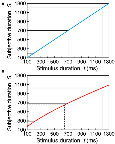
Figure 1. Sample psychophysical functions described by Equation (1). The psychophysical function describes the mapping of objective time (in physical units, e.g., ms) onto subjective time (in arbitrary units). (A) With α = 1, β = 1, and τ = 0, μ is the identity function by which subjective duration equals objective duration. (B) With α = 5, β = 0.75, and τ = −10, μ is a concave function by which durations shorter than t = 654 ms are subjectively perceived longer than they are whereas increasingly longer durations are progressively compressed. Solid black lines illustrate the mapping for sample durations t = 200 ms, t = 1200 ms, and their midpoint at t = 700 ms. Dashed lines in the bottom panel illustrate that, due to the non-linear μ, the midpoint between μ(200) and μ (1200) on the vertical axis does not correspond to the midpoint between t = 200 ms and t = 1200 ms on the horizontal axis.
Semi-objective methods also involve the display of stimuli whose presentation duration varies across trials but observers are not requested to produce quantitative estimates. Instead, they are asked for categorical or comparative judgments. Semi-objective tasks include single-presentation methods and paired-comparison methods. In the former, each trial presents a single stimulus and a categorical response is requested; in the latter, two stimuli are presented in each trial and a comparison is requested. (Multiple-comparison methods involving three or more stimuli per trial will not be discussed here.) Single-presentation methods include the bisection task (asking observers to report whether the currently displayed duration is closer to a short or to a long exemplar repeatedly displayed in a preceding training phase) and the temporal generalization task (asking observers to report whether or not the currently displayed duration is the same as an exemplar duration also repeatedly displayed in a preceding training phase). Paired-comparison methods include the two-alternative forced-choice (2AFC) or comparative task (asking observers to indicate which of the two stimuli in each trial had, say, a longer duration) and the equality or same–different task (asking observers to indicate whether or not the two stimuli had the same duration), although many other variants exist. Almost invariably, semi-objective methods are used to estimate the psychometric function describing how the probability of some response varies with duration (see Figure 2). Landmark points on the psychometric function are subsequently extracted to characterize aspects of time perception, including the bisection point (BP, the 50% point on the psychometric function in a bisection task), the point of subjective equality (PSE, the location of the peak of the psychometric function in the temporal generalization task or the 50% point on the psychometric function in the 2AFC task), or the difference limen (DL, a measure of the spread of a psychometric function). Also often computed is the Weber ratio (WR) defined as either DL/BP or DL/PSE. Superficially, psychometric functions estimated with semi-objective methods offer an account that differs from that provided by psychophysical functions estimated with subjective methods. Yet, the psychometric function embeds the psychophysical function, as will be seen later.
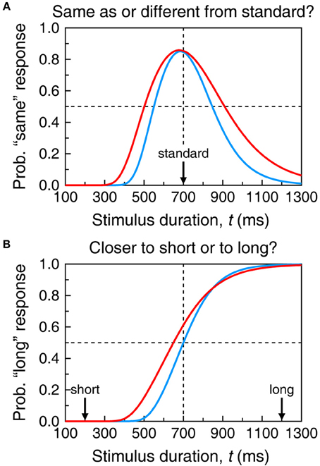
Figure 2. Sample psychometric functions in the temporal generalization task (A) and the temporal bisection task (B). Each function in each panel results from the psychophysical function plotted with the same color in Figure 1, with additional assumptions coming from the models described in sections A Unified Model of Performance across Semi-Objective Psychophysical Tasks and Single-Presentation Methods. Specifically, in the top panel, δ = 150 whereas in the bottom panel, δ = 70 and ξ = 0.5. In both cases γ = 0.15. The red curve in (A) is the same psychometric function plotted in Figure 4A; the red curve in (B) is the same psychometric function plotted with continuous black trace in Figure 5A.
Prospective studies typically include several conditions to investigate differences in subjective time across experimental manipulations (Ulbrich et al., 2007; Wearden et al., 2010; Ogden, 2013) or subject variables (Carlson and Feinberg, 1970; Eisler and Eisler, 1994; Glicksohn and Hadad, 2012). Differences in time perception could naturally be expected to occur as a result of these factors. Our theoretical analyses will assess how the use of alternative semi-objective tasks and the way in which data are analyzed can speak about these differences.
A Unified Model of Performance Across Semi-Objective Psychophysical Tasks
This section presents a unified model of performance in all the semi-objective psychophysical tasks used to investigate time perception. Specific models have been proposed for individual tasks, but they are not always applicable to other tasks and, thus, they offer a fragmentary view of time perception. The model used for our purpose here extends the signal detection theory (SDT) model of Gibbon (1981), which was indeed the basis for most models of performance in semi-objective tasks. The model includes a timing component and a decisional component determining how observers use the outcome of the timing component to make a judgment and give a response.
For the timing component, the model assumes that objective time is internally represented as described by the psychophysical function μ, irrespective of the mechanism by which this representation is obtained. The psychophysical function μ reflects a mapping of objective onto subjective time that can be measured with subjective methods. This does not imply that the psychophysical function estimated with those methods for some particular stimulus should exactly govern the judgments expressed by observers in semi-objective tasks with the same stimulus. Psychophysical functions vary with the subjective method used to estimate them (Carlson and Feinberg, 1970; Angrilli et al., 1997; Gil and Droit-Volet, 2011), but also with instructions (Rattat and Droit-Volet, 2012) or with the interface used to collect responses (Mioni et al., 2014). Yet, judgments reported in semi-objective tasks must arise from a representation of time analogous to that subserving performance in subjective tasks. Extensive research has shown that the psychophysical function for duration is well-approximated by the three-parameter power function
with an exponent β close to unity and a shift τ close to zero. Parameter values vary across stimulus types and experimental conditions (Marks and Stevens, 1968; Fagot, 1975; Eisler, 1976; Dawson and Miller, 1978; Allan, 1983) and one must consider a family μi, in which the subscript (also in the parameters) denotes condition. Within a condition, subjective duration exceeds objective duration within the range of t for which μi(t) > t whereas subjective duration is shorter than objective duration wherever μi(t) <t. Figure 1 showed two psychophysical functions described by Equation (1). If μ(t) = t (Figure 1A), subjective and objective time run identically; if β ≠ 1 (Figure 1B), subjective time runs faster or slower than real time (see Gibbon, 1986, his Figure 1). Across conditions, μi(t) ≠ μj(t) implies that time runs (relatively) faster in one condition than in the other.
The parameters of μ are estimated from the durations reported by observers across repeated presentations of a set of objective durations. The fitted function thus reflects the average subjective duration of a stimulus of duration t. Scalar expectancy theory derived from studies with non-human animals (Church and Deluty, 1977; Gibbon, 1977; Church and Gibbon, 1982) posits that the standard deviation of subjective duration is proportional to the average subjective duration at t, namely,
This is known as the scalar variance assumption or the scalar property. A family of functions σi must also be considered across conditions. With scalar variance, the coefficient of variation σi(t)/μi(t) of the distribution of subjective durations equals γi at all t. Scalar variance holds only approximately in human timing although the standard deviation certainly increases with t (Wearden, 1991b; Lewis and Miall, 2009). In any case, the subjective duration S of a stimulus of duration t under condition i can be regarded as a random variable with mean μi(t) and standard deviation σi(t) and, without loss of generality, S is assumed to be normally distributed (Figure 3). This provides the output of the timing component in the model.
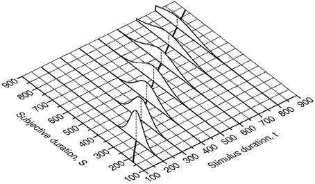
Figure 3. Distributions of subjective duration at selected values of objective duration. The mean of each distribution is given by Equation (1) with the same parameter values used in the bottom panel of Figure 1 (the partly-occluded thick curve on the plane surface shows this psychophysical function). The distributions obey the scalar property in Equation (2) with γ = 0.15.
This characterization implies that the subjective duration elicited by presentation of a stimulus of duration t is a random value sampled from the applicable distribution, regardless of the psychophysical task or the occasion that motivated the presentation of such stimulus. In semi-objective psychophysical tasks, observers are assumed to make a decision and respond according to the values drawn for each of the stimuli presented in each trial. Modeling performance on these tasks thus calls for a decision rule specifying how observers use the current sample (or samples) of subjective duration to make a judgment and give a response. This decisional component must vary across tasks but its elements must be consistent in the sense that the decision rule for some task cannot imply aspects or processes that are explicitly regarded as inexistent or impossible under alternative tasks. This is a reasonable demand on consideration that trials from different tasks can be interwoven in a session, with the response requested on each trial withheld until after stimulus presentation. In such conditions, duration(s) must be internally represented before observers know which decision rule must be used to give a response. Empirical evidence shows that the operation of the stimulus-dependent component precedes and is unaffected by the task-dependent decisional component (Schneider and Komlos, 2008; García-Pérez and Alcalá-Quintana, 2012; García-Pérez and Peli, 2014). On the same grounds, one must assume that μi and σi do not vary across tasks when stimuli and conditions are invariant.
Sections Single-Presentation Methods and Paired-Comparison Methods describe the model (timing output and decision rule) describing performance on the most common semi-objective psychophysical tasks, also discussing other assumptions needed to interpret the data.
Single-Presentation Methods
In single-presentation methods, observers are shown a single stimulus on each trial for them to report a categorical judgment. Making this judgment nevertheless requires that the internal representation of the current stimulus is judged relative to what has sometimes been called an internal standard. The two methods described next differ as to how the internal standard is instated and what type of categorical judgment is requested.
The Temporal Generalization Task
The temporal generalization task consists of a training phase and a test phase. In the training phase, observers are repeatedly shown instances of an exemplar duration tst designated as the standard. The test phase comprises a series of trials each of which displays a duration t around tst and asks observers to indicate whether that duration was the same as tst. A plot of the proportion of “same” responses as a function of test duration describes the empirical psychometric function.
When both phases use the same stimulus and conditions are identical, subjective duration must be governed by the same μ and σ in both phases. Hence, the data are expected to reveal that the test duration at which “same” responses are maximally prevalent is t = tst. But stimuli or conditions may differ across phases: The training phase may use a neutral stimulus such as an oval while the test phase uses emotional stimuli such as angry faces or taboo words. In such case, μ and σ will differ across phases if subjective time runs differently in each condition. Let subscripts “s” and “t” respectively denote the functions that apply to the standard and to the test. Then, one would expect the data to disclose the test duration whose subjective duration equals the subjective duration of the standard. Formally, this is the value tPSE at which μt(tPSE) = μs(tst).
Fitting model-based psychometric functions to the data is useful for these purposes. Formal models from which theoretical psychometric functions for the temporal generalization task can be derived were first proposed by Church and Gibbon (1982) and Wearden (1992). The model described next differs from these in minor respects discussed in section Differences with Previous Models.
Model and assumptions
The training phase helps observers to set an anchor point (internal standard) from the sample of subjective durations elicited by repeated presentation of the standard. The anchor is presumably placed at Sst = μs(tst) and kept invariant. In the test phase, observers compare the random subjective duration S elicited by the current test with Sst and respond according to the magnitude of |S − Sst|. Observers are assumed to have a limited resolution to tell small differences from zero, for otherwise they would always respond “different.” Under these assumptions, the decision rule states that observers respond “same” when |S − Sst| ≤ δ and “different” when |S − Sst| > δ, where δ is the resolution limit and the interval from Sst − δ to Sst + δ is the indifference region.
The mathematical form of the psychometric function for “same” responses is easily derived from these assumptions. Given that Sst = μ (tst) is assumed constant and that S in the test phase is normally distributed with mean μt(t) and standard deviation σt(t), the probability Ψsame of a “same” response varies with test duration t as
where Φ is the unit-normal cumulative distribution function. The psychophysical function μ is thus embedded in the psychometric function, as is the scalar property. Figure 4A shows the psychometric function when μs = μt ≡ μ and σs = σt ≡ σ (see the legend for parameter values) so that Equation (3) becomes
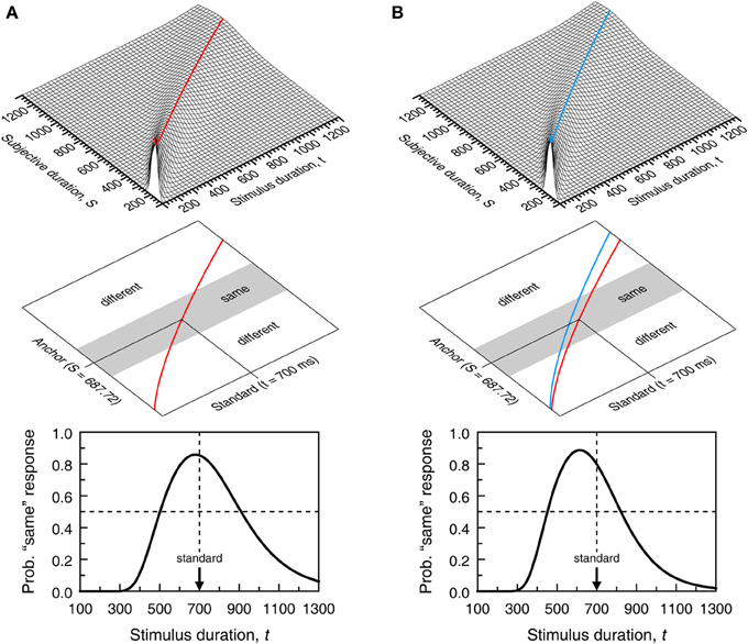
Figure 4. Model-based psychometric functions for the temporal generalization task. In (A), perception of duration is governed by the same psychophysical function for training and test stimuli; in (B), they are governed by different psychophysical functions. The top panel shows a continuous version of the surface for which cross-sectional plots at selected t were shown in Figure 3. The surface in (A) has the same parameters as in Figure 3 and governs perception of duration for the training stimulus in both columns and also for the test stimulus in (A); the surface in (B) only differs in that α = 5.4 instead and is assumed to govern perception of duration of the test stimulus in (B). The middle panel shows the partition of decision space into a central gray region of subjective durations that result in “same” responses and two outer white regions of subjective durations that result in “different” responses. The central gray region spans δ = 150 units on either side of the anchor point. The bottom panel shows the resultant psychometric function in Equation (3). The ordinate at each value of t equals the area under the cross-section at t of the surface in the top panel within the region that results in “same” responses.
Even in these conditions, Ψsame does not peak at the standard duration because t = tst maximizes Equation (4) only when σ(t) is a constant function independent of t. When σ(t) obeys the scalar property, Equation (4) peaks at . The right-hand side of this expression evaluates to 0.99Sst when γ = 0.1 and to 0.92Sst when γ = 0.3, but the spacing used in empirical studies (typically 100–200 ms) is too coarse to reveal this shift. If differences in stimuli or conditions across training and test phases affect subjective time, Ψsame is further shifted because the peak of Equation (3) is further away from t = tst when μs ≠ μt (see Figure 4B). Note also that differences between σs and σt are inconsequential, as σs plays no role in Ψsame. The gradients on either side of Ψsame are determined by how σt varies with t. With scalar variance, Ψsame is positively skewed. The skew is further emphasized when μt is a concave function (βt < 1 in Equation 1) and reduced or even reversed when μt is convex (compare the two curves in Figure 2A).
Because Ψsame does not peak at t = tst even when μs = μt, observed shifts of Ψsame away from tst cannot be interpreted as evidence that μs ≠ μt and, thus, of differences in subjective time in the conditions of the test phase relative to the training phase. Other difficulties in the interpretation of data from the temporal generalization task will be discussed in section Summary and Discussion of Single-Presentation Methods.
Differences with previous models
Wearden (1992) proposed three variants of the model of Church and Gibbon (1982), which are discussed next in our notation. All variants share two characteristics: (1) subjective duration is assumed accurate on average so that the psychophysical function is μ (t) = t in all cases and (2) the internal standard is not regarded as a fixed value but as a random variable with mean tst. Also, the resolution parameter (called threshold by Wearden) is fixed at δ in some variants but regarded as random with mean δ in others. All three variants use a decision rule analogous to that in section Model and Assumptions and they differ as to the assumed variances of subjective duration, internal standard, and threshold (when random).
The modified-Church-and-Gibbon (MCG) model assumes σ(t) = 0. Thus, subjective duration is not a random variable and, given μ(t) = t, it is identical to objective duration. This model places the scalar property at the internal standard (drawn in each trial from the memory representation of the standard) whereas the threshold is regarded as a random variable with fixed variance. The MCG model is structurally equivalent to our model because the distribution of |X − Y| is the same regardless of which of X or Y is the random variable and which is the constant and also because the variability of δ can be formally transferred to the internal standard. But this model presents an empirical difficulty: If subjective duration equals objective duration (a consequence of assuming μ(t) = t and σ(t) = 0), observers would be perfectly accurate in paired-comparison tasks asking them to judge the relative durations of two stimuli displayed in each trial (see section Paired-Comparison Methods).
The fixed-threshold model removes the variability of δ while leaving other assumptions of the MCG model intact. This model is also formally equivalent to our model and to the MCG model, and results reported by Wearden (1992; see his Table 1) reveal that the estimated variability of the internal standard increases under this model to capture the variability attributed to threshold under the MCG model. Finally, the timing-variability model assumes scalar variance for subjective duration in place of σ(t) = 0, also assuming scalar variance with the same γ for the internal standard and a threshold randomly drawn in each trial from a distribution with fixed variance. Structurally, this model is not equivalent to the others because it involves a ratio of independent normal random variables, whose distribution is not normal (Simon, 2002, formula 7.7). The model nevertheless produces nearly identical psychometric functions and is also functionally equivalent to the previous two and to our model, although scalar variance affects two random variables here and must result in smaller estimates of γ to account for the same data (see Table 1 in Wearden, 1992).
Because all the models of Wearden (1992) use μ(t) = t, they explicitly assume that subjective and objective time run identically and, hence, the models are incompatible with the notion that subjective time may run at a different pace, or with an interest in assessing what that pace may be and how it varies across conditions. Fitting these models to empirical data enforces the assumption of veridical time perception and succeeding at that shows that temporal generalization data are compatible with the notion that subjective time is equivalent to objective time. This outcome is not to be taken as a proof that time perception is never distorted relative to objective time but as a manifestation of non-identifiability issues hampering the interpretation of data, whose discussion is deferred to section Summary and Discussion of Single-Presentation Methods.
The Temporal Bisection Task
The temporal bisection task also consists of a training phase and a test phase. In the training phase, observers are shown repeated instances of exemplar durations tshort and tlong designated short and long, respectively. The test phase comprises trials displaying a test duration t typically between tshort and tlong. Observers are asked to judge whether the current test duration is closer to the short or to the long exemplars. A plot of the proportion of “long” responses at each test duration describes the empirical psychometric function and the 50% point on this function is taken to be the BP.
Performance is governed by common μ and σ if stimuli and conditions do not differ across phases. The BP might then be expected to lie at the midpoint between tshort and tlong only if μ is linear (Figure 1A and the blue curve in Figure 2B). With non-linear μ, the objective midpoint does not map onto the subjective midpoint (Figure 1B) and the BP would be expected to lie at the test duration associated with the subjective midpoint (red curve in Figure 2B). Note that the two cases in Figure 2B reflect an exquisite ability to bisect the subjective continuum; the different BPs simply reflect the form of μ. Bisection tasks are also used with different stimuli or conditions in the training and test phases so that μt may differ from μs and σt may differ from σs (using the same notation as before). In such cases, one expects the BP to identify the test duration that is subjectively midway between the subjective durations of the short and long standards.
Quite often, cumulative Gaussian or logistic functions are fitted to data to estimate the BP and the DL from location and slope parameters. Formal models from which suitable psychometric functions can be derived were first proposed by Gibbon (1981) and Wearden (1991a; see also Wearden and Ferrara, 1995). The model described next differs from these in some respects discussed in section Differences with Previous Models.
Model and assumptions
The training phase helps observers to set anchor points from the sample of subjective durations elicited by repeated presentation of short and long exemplars. In principle, the anchor points are assumed to be placed at Ss = μs(tshort) and Sl = μs(tlong) and also to be invariant. In the test phase, observers compare the subjective duration S of the current stimulus with Ss and Sl and respond according to which of |S − Ss| or | S − Sl| is the smallest. In principle, “long” responses are in order when |S − Sl | < |S − Ss|, which simplifies to S > (Ss + Sl)/2. For all purposes, this is as if observers set a single anchor at the subjective midpoint Smp = (Ss + Sl)/2. Assuming that observers use a point criterion and always classify S as closer to the short or the long exemplars is incompatible with assumptions in the model for temporal generalization: If observers can use a point criterion in the bisection task to decide whether S is above or below Smp, they should show the same capability in the temporal generalization task for deciding whether S is above or below Sst, and thus they would always respond “different.” Observers surely have limited resolution also in the bisection task so that they respond “short” when S < Smp − δ, respond “long” when S > Smp + δ, and cannot tell when Smp − δ ≤ S ≤ Smp + δ, also involving a resolution limit and an indifference region. But, because observers are forced to respond “short” or “long,” they must use an extra criterion when they cannot tell. The model assumes that they respond “long” with probability ξ, reflecting their response bias and regardless of the criteria that render such outcome.
The psychometric function Ψlong for “long” responses is easily derived from these assumptions. Since Smp is assumed constant and S in the test phase is normally distributed with mean μt(t) and standard deviation σt(t), the probability of a “long” response varies with test duration t as
Figure 5A shows sample psychometric functions when μs = μt = μ and σs = σt = σ for several values of the response bias parameter ξ. It is noteworthy that the location of the 50% point on Ψlong varies greatly with ξ. In principle, only when μs and μt are linear does tmp map onto Smp (Figure 1). But, even when they are linear, Ψlong has its 50% point at tmp only when ξ = 0.5 (blue curve in Figure 2B). It is also noteworthy that the location and slope of Ψlong are greatly affected by the irrelevant response bias and resolution parameters ξ and δ (compare with the dashed black curve for δ = 0 in the bottom panel of Figure 5A), undermining interpretation of the BP and the DL.
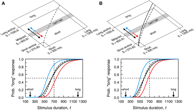
Figure 5. Model-based psychometric functions for the temporal bisection task. Panels (A,B) reflect the same scenarios as in Figure 4 regarding psychophysical functions (identified in the top panels here as dashed and solid curves instead of red and blue curves). The top panel shows a decision space analogously partitioned (now using δ = 70) but the regions now result in “short,” “I can't tell,” and “long” judgments although “I can't tell” judgments must still be reported as “short” or “long” responses. The bottom panel shows the psychometric functions (from Equation 5) that may result according to how observers respond when undecided. The blue curve arises when “I can't tell” judgments are always reported as “long” responses (blue arrow in the top panel; ξ = 1 in Equation 5); the red curve arises when “I can't tell” judgments are always reported as “short” responses (red arrow in the top panel; ξ = 0 in Equation 5); the black curve arises when “I can't tell” judgments are reported as “short” or “long” responses with equiprobability (double-headed black arrow in the top panel; ξ = 0.5 in Equation 5); the dashed curve arises if δ = 0 so that observers use a point criterion at the subjective midpoint and are never undecided.
If differences in stimuli or conditions across training and test phases affect subjective time, Ψlong is further shifted (Figure 5B) although given the influence of response bias, the 50% on Ψlong carries no information that can be readily interpreted in terms of the pace of subjective time. As in temporal generalization, differences between σs and σt are inconsequential as σs plays no role in Ψlong. As resolution decreases (i.e., δ increases) with fixed ξ, Ψlong becomes shallower (compare the dashed and solid black curves in the bottom panels of Figure 5). Finally, Ψlong is not symmetric about its 50% point: Its left side rises more sharply than its right side levels off. This is due to the scalar property (for a discussion of this issue, see Killeen et al., 1997).
It is worth mentioning a mixed task in which a standard is used in the training phase (as in temporal generalization) and observers report whether the current test duration is longer or shorter than the standard (as in temporal bisection). In such case (Grondin and Rammsayer, 2003), observers do not need to build Smp from Ss and Sl in the training phase but build Sst directly and use it in the test phase. The model psychometric function is still given by Equation (5) with Sst in place of Smp. Another variant of the bisection task is the “partition bisection” of Wearden and Ferrara (1995), in which the training phase is omitted and observers are simply asked to classify test stimuli as “short” or “long” using whichever criterion they wish. The psychometric function is again given by Equation (5), except that Smp is a free parameter that captures the arbitrary criterion used by observers. In yet a further variant, observers receive feedback relative to the objective midpoint of the range of test durations (Grondin, 1998), which should help them to set a stable criterion.
Differences with previous models
The seminal model of Gibbon (1981) is analogous to the model just described except that he omitted the indifference region. His model thus arises by setting δ = 0 to revert to a point criterion. Gibbon analyzed versions of the model in which μ is non-linear and σ obeys the scalar property so that estimated model parameters speak of the pace at which subjective time runs. In addition, he considered the implications of decision rules involving point criteria other than Smp = (Ss + Sl)/2.
Wearden (1991a) adapted his fixed-threshold model of temporal generalization for application to bisection tasks, thus including the indifference region missing in Gibbon's (1981) model. In this model, observers draw random memories of the long and the short durations (both of which are accurate on average and have scalar variance) to compare them with the exactly perceived test duration (i.e., μ(t) = t and σ(t) = 0), responding “long” or “short” according to which distance is the smallest but provided that the difference of distances is beyond a fixed threshold (resolution limit). On trials in which the threshold is not exceeded, observers are undecided and always respond “long.” This model is formally equivalent to our model in Equation (5) with ξ = 1, μt(t) = t, and σt(t) reflecting instead the variability of the memory representations. Wearden and Ferrara (1995) later made two amendments to this model: Undecided observers respond “short” or “long” with equiprobability (ξ = 0.5) and the anchor Smp is randomly drawn in each trial from a distribution whose mean equals the average of the set of test durations. This is the only random variable in the model but Wearden and Ferrara's (1995) writing is unclear about whether its standard deviation was fixed or increased with t so as to incorporate the scalar property.
By embedding the assumption that μ(t) = t, these models are unsuitable for assessing how subjective time runs compared to objective time. A 50% point found to be away from tmp is implicitly attributed to response bias or to a criterion Smp placed away from μs(tmp) = tmp (for an amendment of the model in this respect, see Wearden, 2004). Such decisional or response aspects are unrelated to time perception, which is regarded as accurate under these models. The same holds for the model of Killeen et al. (1997), which also assumes μ(t) = t and the scalar property but uses a logistic function as an approximation to Φ.
Kopec and Brody (2010) presented a model of an entirely different nature for the bisection task. This model is not considered here because it involves assumptions, processes, and decision rules that are specific to bisection tasks and cannot describe performance in any other task. For instance, applied to a temporal generalization task, the model posits that Ψsame should have a symmetric Gaussian shape peaking at t = tst and such that Ψsame(tst) = 1.
Summary and Discussion of Single-Presentation Methods
Psychometric functions describing performance in single-presentation methods embed a representation of subjective duration (the functions μ and σ) and decisional aspects pertaining to how judgments are made and reported (the anchor points Sst or Smp, the observers' resolution δ and, where applicable, their response bias ξ). All of these components affect the psychometric function, including its location and slope. With reasonable assumptions about these components, Figures 4, 5 showed that neither the empirical location of the peak of Ψsame and its gradient on either side nor the empirical location of the 50% point on Ψlong and its slope can be interpreted as pure indices of timing processes. But the interpretation of data is further complicated if three other implicit assumptions of single-presentation methods are violated.
The first assumption is that the indifference region is symmetric about the anchor point. In general, boundaries might be placed at Sst − δ1 and Sst + δ2 in the temporal generalization task (or at Smp − δ1 and Smp + δ2 in the bisection task), with symmetry occurring when δ1 = δ2 = δ. The effects of an asymmetric region are illustrated in Figure 6: Psychometric functions shift as a result of this decisional bias. Obtaining direct evidence of the symmetry of the indifference region is impossible with single-presentation data, but methods allowing this determination exist and their use has revealed that the indifference region is generally asymmetric (García-Pérez and Alcalá-Quintana, 2013; García-Pérez and Peli, 2014).
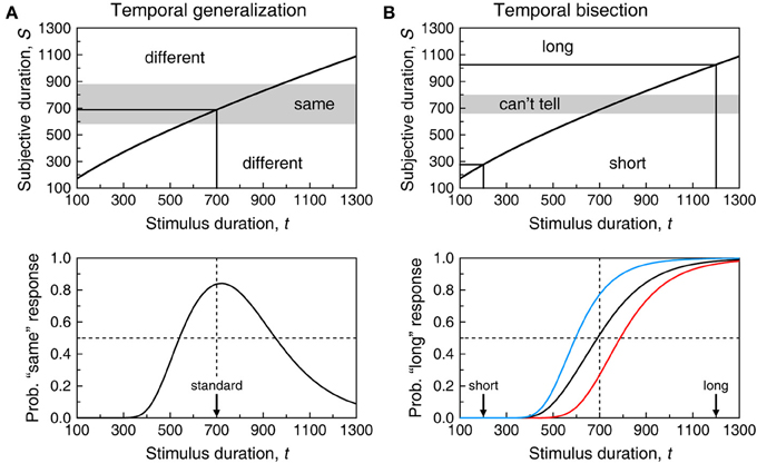
Figure 6. Effects of decisional bias in the temporal generalization (A) and temporal bisection (B) tasks. Graphical conventions as in Figures 4, 5. Decisional bias shows in that the central region for “same” or “I can't tell” judgments is displaced upwards by 30 units relative to its location in Figure 4 or 5. Psychometric functions are accordingly shifted laterally to the right.
The second assumption is that the anchor points Sst and Smp are respectively placed at μs(tst) and at (μs(tshort) + μs(tlong))/2 during the training phase, as if observers used the arithmetic mean of a large sample of subjective durations elicited by repeated presentation of the standard (or the short and long exemplars). If the anchor were placed elsewhere during the training phase, the decision criterion during the test phase would not be at its presumed location and Ψsame (or Ψlong) would shift accordingly. In these conditions, shifts of the psychometric function do not necessarily reflect differences in subjective time across training and test phases even if μs(t) ≠ μt(t) ≠ t. Obtaining evidence as to where the anchor point was placed seems impossible.
The third assumption is that anchors presumably placed at Sst = μs(tst) or Smp = (μs(tshort) + μs(tlong))/2 are stable. If they drifted systematically during the test phase, aggregating data across the session would shift the psychometric function. Concerns that anchor drift may occur come from adaptation level theory (Helson, 1948), which posits that the set of durations used during the test phase defines a context that relocates the internal standard. Stimulus range effects on temporal generalization do not seem to have been studied in a way that allows determining observable consequences on the location of Ψsame, but these effects have been reported for the bisection task (Wearden and Ferrara, 1995, 1996; Penney et al., 2014). The model of Wearden and Ferrara (1995) assumes that, as a result of this, the anchor is placed at the arithmetic mean of the set of test durations (or at 95% of this value; see Wearden, 2004). But the dynamics of the underlying processes are unknown, which precludes devising ways to eliminate or compensate for their effects so that bisection data are not contaminated by criterion placement.
These difficulties undermine the interpretation of temporal generalization and bisection data even under identical conditions in the training and test phases. Consider the bisection results reported by Gil et al. (2009). The training phase used a picture of an oval with tshort = 400 ms and tlong = 1600 ms so that tmp = 1000 ms. Among conditions involving pictures of liked and disliked foods, the test phase also included a condition with the oval picture. Averaged across observers, results with the oval showed a remarkable shift: Ψlong had its 50% point at t ≈ 800 ms, with Ψlong(tmp) ≈ 0.8. Assuming μs = μt = μ, σs = σt = σ, incorporating the scalar property, and removing the indifference region (i.e., δ = 0), Equation (5) reduces to Ψlong(t) = Φ (γ − Smp/σ(t)). If Smp = μ(tmp) and τ in Equation (1) is removed, Ψlong(t) = Φ(γ − tβmp/γtβ) obtains. Reproducing the shape described by data from the oval condition in Gil et al.'s Figure 2 with this function requires β ≈ 2.39 and γ ≈ 1.46, unreasonable values compared to common estimates of β in μ and γ in the scalar property. Data are nonetheless unquestionable and a 50% point at t ≈ 800 ms with Ψlong(tmp) ≈ 0.8 are empirical facts. What is less clear is what the data say about the relation of subjective to objective time, or whether time is under- or over-estimated as opposed to veridically perceived. The same data could have arisen if β = 1 (i.e., μ(t) = t) and the assumption that Smp = μ (tmp) is removed, implying that observers perceive duration veridically but for some reason they do not set the anchor at μ(tmp) during the training phase (Raslear, 1985; Allan and Gerhardt, 2001; Allan, 2002a,b). And the same shift could have been caused also with μ(t) = t and by reinstating the assumption that Smp = μ (tmp) if observers had a non-null indifference region (i.e., δ ≠ 0) and responded with bias when undecided (Figure 5). Which scenario is responsible for the observed results is indiscernible because all account for the data equally well.
It is remarkable that virtually all analyses of bisection data have explicitly or implicitly assumed μt(t) = t and, hence, that duration is accurately perceived. Yet, what should have thus been regarded as criterion shifts or response bias has been inconsistently interpreted as evidence of differences in perceived duration. To see that the assumption of veridical time perception is implicit when two-parameter psychometric functions are fitted to bisection data, make δ = 0 (i.e., a point criterion), μt(t) = t (i.e., veridical time perception), and σt(t) = k (i.e., remove the scalar property). In these conditions, Equation (5) becomes Ψlong(t) = Φ ((t − Smp)/k), which is the widespread cumulative Gaussian fitted to bisection data and sometimes replaced for convenience with a logistic function. On fitting this psychometric function to data, Smp is regarded as a free parameter to account for observed shifts with respect to tmp, but this is synonymous with observers using an arbitrary criterion that varies across conditions (i.e., they do not set Smp at tmp in all conditions) and perceived duration being veridical and invariant across conditions (since μt(t) = t in all cases).
Interpretation of bisection data is more difficult when the test phase does not include a condition with the training stimulus. Consider the results reported by Tipples (2010). Stimuli in the training phase were eight-consonant strings with tshort = 400 ms and tlong = 1600 ms so that tmp = 1000 ms. The test phase used words of six different types: high arousal negative or positive, low arousal negative or positive, neutral, and sexual taboo. Since the 50% point on Ψlong was 30–40 ms higher for taboo words than for the other types of word, Tipples concluded that time flies when one reads taboo words. Yet, and leaving other issues aside, without a reference provided by the 50% point on the psychometric function for eight-consonant strings, the 50% point on Ψlong for test words is uninterpretable: The conclusion would have differed if the 50% point on Ψlong for eight-consonant strings were above that for taboo words or below that for the other types of word. Tipple's conclusion is even more puzzling on consideration that, on average across observers, the 50% point lay between 955 and 970 ms for non-taboo words and nearly at 1000 ms for taboo words (see his Figure 2). Since tmp = 1000 ms, the conventional (though unwarranted) conclusion should have been that time is perceived accurately only with taboo words.
These considerations apply also to the temporal generalization task, although studies assessing if time flies or slows down under certain conditions have almost exclusively used the bisection task. Measuring the psychometric function (be it Ψlong or Ψsame) for training stimuli sets a reference for comparison with the psychometric function for other types of stimuli, but this does not solve the problems of single-presentation methods. The multiplicity of factors that can shift the psychometric function away from tmp (or tst) preclude the interpretation of observed shifts as evidence of differences in subjective time across conditions. Bisection tasks are more seriously affected by this problem because response bias further alters the slope of the psychometric function (Figure 5) and contaminates DL estimates.
One might think that these problems would be solved by fitting psychometric functions such as those in Equations (3) or (5) to the data. Replacing the assumption of symmetry built into them (i.e., using δ1 and δ2 as needed instead of the single δ in them) puts into the fitted function all the factors that contribute to observed performance. Estimated parameter values would thus provide all the information needed for a proper interpretation of the data. With a psychophysical function given by Equation (1), estimates of the exponent β would directly indicate how time runs in each experimental condition provided the condition used to set the anchors is also tested. Unfortunately, models for single-presentation tasks are non-identifiable: There are infinite sets of parameter values that produce the same psychometric function (Yarrow et al., 2011; García-Pérez and Alcalá-Quintana, 2013; García-Pérez and Peli, 2014). This is not a problem of the models, but an indication that the intervening factors are inextricably confounded in single-presentation data. Data gathered with single-presentation methods are simply uninterpretable. Luckily, paired-comparison methods offer a suitable and dependable alternative with which these influences can be separated out.
Paired-Comparison Methods
Trials in paired-comparison methods display two stimuli (a standard and a test, both of which may vary across trials) for observers to make a comparative judgment. Single-presentation methods imply a comparison too, but with respect to an internal standard. In paired-comparison tasks, the standard is explicit and subject to the same type of processing as is the test. A training phase is not needed to instate an internal standard, nor are assumptions about its placement and stability. Some modifications of the temporal generalization and bisection tasks turn them into paired-comparison methods, and the models discussed here apply to them too. For instance, the roving standard task of Allan and Gerhardt (2001) or Rodríguez-Gironés and Kacelnik (2001) presents in each trial a short and a long exemplar (which vary across trials) so that observers compare the test duration with the current exemplars. Similarly, the episodic temporal generalization task of Wearden and Bray (2001) presents a variable standard in each trial which is the reference for the observers' current judgment.
In paired-comparison trials, standard and test elicit subjective durations from the applicable distributions and observers judge by comparing the values drawn in the current trial. Observers can be asked to report whether both stimuli have the same subjective duration (the equality task), whether the first or the second appeared to have a longer duration (the comparative task), or whether the first, the second, or neither was subjectively longer than the other (the ternary task, which blends the two other tasks). [Incidentally, the bisection task can also be administered in a ternary format (Droit-Volet and Izaute, 2009) and its application reveals an indifference region whose width and symmetry differs across observers (García-Pérez and Peli, 2014).] The outcome of the timing component of a psychophysical model of performance in paired-comparison tasks cannot vary with the question asked at the end of the trial, as discussed in section A Unified Model of Performance across Semi-Objective Psychophysical Tasks. The next section describes the model for paired-comparison tasks, including a common timing outcome and a decision rule that varies with the task.
The Model for Paired-Comparison Judgments
The model is analogous to an indecision model derived from SDT for use in other psychophysical tasks (García-Pérez and Alcalá-Quintana, 2010a,b, 2011a,b, 2013; Alcalá-Quintana and García-Pérez, 2011; García-Pérez and Peli, 2014). Its relation to other models will be discussed in section Differences with Previous Models. In the general case when standard and test differ qualitatively (as might be when test and standard are, e.g., eight-consonant strings vs. taboo words, or pictures of an oval vs. pictures of liked foods), the subjective duration Sst of a standard duration tst is normally distributed with mean μs(tst) and standard deviation σs(tst) whereas the subjective duration St of a test duration t is normally distributed with mean μt(t) and standard deviation σt(t). Sample psychophysical functions that differ across test and standard stimuli are shown in the two right panels of Figure 7A. When standard and test stimuli are the same or when their differences do not affect subjective duration, μs = μt and σs = σt (two left panels of Figure 7A). Our goal here is to derive the psychometric function relative to a standard of fixed duration tst across trials, whether or not such trials are interwoven with trials for other standards (which will define separate psychometric functions).
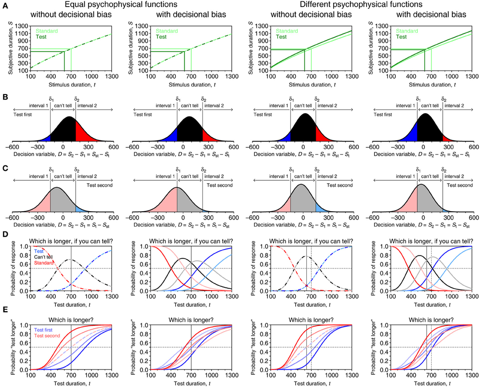
Figure 7. Model-based psychometric functions for paired-comparison tasks in four different scenarios. (A) Psychophysical functions μs (light green) and μt (dark green). In the two columns on the left, μs = μt with αs = αt = 5, βs = βt = 0.75, and τs = τt = −10 in Equation (1); in the two columns on the right μs is as before but parameters of μt are αt = 5.4, βt = 0.75, and τt = −10. Scalar variance is assumed with γs = 0.15 in all cases and γt = 0.15 also in the two left columns but γt = 0.10 in the two right columns. Light and dark green lines show in each scenario the mapping of the standard at tst = 700 ms and a sample test at t = 600 ms. (B) Distribution of the decision variable for the standard-test pair just mentioned in a trial in which the test is presented first. The distribution is narrower in the two columns on the right due to the smaller variance. The decision space is partitioned into three regions by vertical lines at D = δ1 and D = δ2, with δ1 = −150 and δ2 = 150 in the first and third columns (i.e., no decisional bias) but δ1 = −70 and δ2 = 230 in the second and fourth columns (i.e., decisional bias). Each region is associated with the judgment indicated at the top, and the probability of the corresponding judgment equals the area under the distribution in that region. (C) Distributions in a trial involving the same pair but with the test presented in the second interval. (D) Psychometric functions in the ternary task for each presentation order. Color codes relate to (B,C) (e.g., dark blue denotes “interval 1” responses when the test was presented first; pale blue denotes “interval 2” responses when the test was presented second). A thin vertical line indicates the true location of the PSE defined as tPSE = μ−1t (μs (tst)). With parameters given above, tPSE = 700 ms in the two columns on the left whereas tPSE = 630.8 ms in the two columns on the right. (E) Psychometric functions for “test longer” responses in the comparative task for each presentation order and with response bias ranging from ξ = 0.5 (paler curves) through ξ = 0.75, to ξ = 1 (darker curves). The location of the true PSE is also indicated in each panel by a thin vertical line.
The model assumes that Sst and St are independent from one another and that observers' judgments are based on the magnitude of a decision variable D = S2 − S1 computed from the subjective durations of the second and first stimuli in the current trial. (The direction in which the difference is computed is immaterial, as will become evident below.) Because test and standard can (and should) be presented in either order with equal frequency across trials, each presentation order must be considered separately. Thus, on trials in which the test is presented first, D = Sst − St is normally distributed with mean μs(tst) − μt(t); on trials in which the test is presented second, D = St − Sst is also normally distributed but with mean μt(t) − μs(tst). In both cases the variance of D is the sum of the variances of Sst and St. Figures 7B,C show the distributions of D for each presentation order on a trial with t = 600 ms when tst = 700 ms, given the psychophysical functions in Figure 7A. Limited resolution also prevents observers from using a point criterion and the decision space is partitioned into three regions separated by boundaries δ1 and δ2, which are symmetric about D = 0 when δ1 = −δ2 (first and third panels in Figures 7B,C) and otherwise reflect a decisional bias (second and fourth panels in Figures 7B,C). Judgments turn into responses in a way that varies with the task.
Consider first a ternary task in which observers report whether duration was subjectively longer in the first interval, in the second, or in neither. Observers respond “interval 2” when D > δ2, “interval 1” when D < δ1, and “I can't tell” when δ1 ≤ D ≤ δ2 (see labels in the top part of Figures 7B,C). Response probabilities vary with presentation order due to the different mean of D in each case. Specifically, the probability Ψi of an “interval i” response when the test is presented in interval i, with i ∈ {1, 2}, varies with t as
the probability ϒi of an “I can't tell” response when the test is presented in interval i varies with t as
and the probability of responding as the interval in which the standard was presented is 1 − Ψi − ϒi. Figure 7D plots psychometric functions in each scenario and their features are discussed next.
The most conspicuous aspect is that psychometric functions do not differ across presentation orders in the absence of decisional bias (first and third columns in Figure 7) and they differ otherwise (second and fourth columns in Figure 7). Differences (or lack thereof) in the psychophysical functions for standard and test also have observable effects. Consider the PSE as a proxy to these differences. By definition, the PSE is the duration t that the test must have for its subjective duration to equal the subjective duration of the standard. Thus, the PSE is the duration tPSE = μ−1t (μs (tst)) and its location is readily identifiable in the psychometric functions. Consider the left column of Figure 7, where δ1 = −δ2 and tPSE = tst because μs = μt. Here, Ψ1 (blue curve) crosses 1 − Ψ2 − ϒ2 (pale red curve) at t = tst and Ψ2 (red curve) also crosses 1 − Ψ1 − ϒ1 (pale blue curve) at that point. It can be easily seen from Equations (6) to (7) that these crossings occur under any conditions at the duration t satisfying μt(t) = μs(tst). In contrast, ϒ1 and ϒ2 (black and gray curves) peak below t = tst due to the scalar property. Hence, “I can't tell” responses are not maximally prevalent at the PSE and, thus, it is not the location of the peak of ϒ1 or ϒ2 that signals the PSE.
With decisional bias under the same conditions (second column in Figure 7), psychometric functions differ across presentation orders but the PSE is identically encoded because the crossing property holds always. In contrast to the preceding case, where ϒ1 and ϒ2 superimpose, their crossing here also occurs at the PSE. It can again be easily seen from Equations (7) that ϒ1(t) = ϒ2(t) at all t when δ1 = −δ2 (the conditions in the first column of Figure 7) and that they cross at the duration t satisfying μt(t) = μs(tst) when δ1 ≠ −δ2 (the conditions in the second column of Figure 7). The third and fourth columns in Figure 7 show that identification of the PSE is also not hampered when μs ≠ μt and σs ≠ σt, as would occur when subjective time runs differently for test and standard. In the absence of decisional bias (third column), the crossing occurs at t = μ−1t (μs (tst)) = 630.8 ms (thin vertical line); with decisional bias (fourth column), the crossings still occur at the same location. In sum, in the ternary paired-comparison task, the effects of decisional bias are not confounded with those of psychophysical functions that differ for standard and test. In this task, the “I can't tell” option also eliminates the contaminating influence of response bias because observers are not forced to give uninformative “interval 1” or “interval 2” responses when undecided.
The equality task, where observers report whether or not the two durations are subjectively equal, renders analogous outcomes. Observers respond “same” when they would have responded “I can't tell” in the ternary task whereas they respond “different” when they would have responded “interval 1” or “interval 2.” The psychometric functions in Equations (7) hold for the equality task, and the preceding discussion applies also to this task. It should be noted that the PSE is not identifiable by eye in ϒ1 and ϒ2 in the absence of decisional bias (i.e., when δ1 = −δ2 and the functions superimpose). This is not a problem, as will be discussed in section Summary and Discussion of Paired-Comparison Methods.
In contrast, the comparative task in which observers are forced to respond “interval 1” or “interval 2” calls again for a response bias parameter ξ describing how observers give arbitrary responses when they cannot tell which duration was longer. It should be clear by now that this can only bring complications. Assume that, as a result of response bias, observers respond “interval 2” with probability ξ when they cannot tell. In this task, “interval i” responses are translated as “test longer” when the test had been presented in interval i. The probability Ψi of “test longer” responses when the test was presented in interval i varies with t as
These psychometric functions are plotted in Figure 7E for sample values of ξ in each of the same four scenarios. The PSE is still defined with respect to the underlying psychophysical functions, but Figure 7D shows that the 50% point on the psychometric function does not relate to this definition. Consider again the first column of Figure 7, in which psychophysical functions are identical for test and standard and there is no decisional bias. The psychometric functions are identical for both presentation orders only when ξ = 0.5 (dashed curves) and their 50% point lies at the true PSE in such case; as ξ increasingly exceeds 0.5, Ψ1 (blue curves) shifts progressively to the right whereas Ψ2 (red curves) shifts progressively to the left, with their 50% points symmetrically placed with respect to the PSE. Both functions also turn progressively steeper in this transition and it is also clear that Ψ1 and Ψ2 have different shapes (i.e., they do not differ by translation only), which is another consequence of the scalar property. In the third column of Figure 7, still without decisional bias but when psychophysical functions differ for test and standard, the psychometric functions are displaced laterally toward the true PSE, maintaining the properties described above. Yet, with decisional bias (second and fourth columns), lack of response bias (ξ = 0.5) produces psychometric functions that also differ across presentation orders, although Ψ1 and Ψ2 still have their 50% points symmetrically placed around the true PSE.
Data from the comparative task are usually aggregated across presentation orders, although this practice is unadvisable (Ulrich and Vorberg, 2009). The resultant psychometric function is then Ψ2AFC(t) = (Ψ1(t) + Ψ2(t))/2 and it is easy to see from Equations (8) that the 50% point on Ψ2AFC occurs at t = μ−1t (μs (tst)). Thus, the average of the psychometric functions for each presentation order has its 50% point at the PSE, a result derived by Ulrich and Vorberg for the case in which μs = μt and generalized by García-Pérez and Alcalá-Quintana (2010a, 2011b) for the case in which μs ≠ μt and tPSE ≠ tst. Although data from the comparative task are still useful for estimating the PSE, estimation of the true DL from percent points on the psychometric function is impossible due to the strong influence of response bias on its slope.
Differences with Previous Models
Models for paired-comparison tasks are used in many areas of psychophysics. Almost all of them derive from SDT principles and share structural characteristics with our model, except that they do not include an indifference region (i.e., they assume δ1 = δ2), nor are they adapted to ternary tasks. With δ1 = δ2 = 0, Equations (8) become
Such model does not seem to have been used in time perception. Conventional practice fits instead cumulative Gaussian or logistic functions to the data or, equivalently, fits straight lines to the z-scores of observed proportions. This entails a model analogous to (and with the same problems as) the model discussed in section Summary and Discussion of Single-Presentation Methods for bisection data. In the comparative task, the argument of the sigmoidal function is also of the form (t − a)/b and the consequences are identical: The free location parameter a replaces μs(tst) in Equation (9) and allows the 50% point to be placed as needed without connection to the subjective duration of the standard; the free spread parameter b replaces the entire denominator of the argument of Φ in Equation (9), thus removing the scalar property; and replacement of μt(t) with t amounts to assuming that subjective and objective time run identically. Succeeding in fitting such sigmoidal function and observing differences in estimated location parameters across conditions can only be justifiably interpreted as criterion shifts.
In contrast, a model proposed by Rammsayer and Ulrich (2001) does justice to the assumptions and goals of studies on time perception. In their model, consideration of the statistics of counting processes yielded a non-identity psychophysical function and subjective durations whose standard deviation increases with t. The model was also developed for application to the ternary task used to gather their empirical data. With appropriate replacements for μ and σ, their model and the resultant psychometric functions for the ternary task are identical to those in Equations (7) and (8) above except that Rammsayer and Ulrich set δ1 = −δ2 (i.e., no decisional bias). For unknown reasons, this model was subsequently abandoned by their proponents, as was the ternary task.
Another model for the comparative task was proposed by Dyjas et al. (2012). Again in comparison with our model, they assumed no indifference region (i.e., δ1 = δ2 = 0), undistorted time perception (i.e., μt(t) = μs(t) = t), non-scalar timing (i.e., σt(t) = σs(t) = σ, a constant), and a history component that alters an “internal standard” in line with adaptation level theory. The internal standard is updated on every trial as the convex sum of its value on the previous trial and the subjective duration of the first interval in the current trial. Such internal standards can be described as normally distributed with mean μs(tst) = tst and a standard deviation that varies with presentation order (see expressions for their variances in Equations 12–13 and 15–16 of Dyjas et al.). For simplicity, let σ1 and σ2 represent the equivalent standard deviation of the internal standard when the test is presented first or second. All of this turns Equations (8) into
We use the term “equivalent” because substituting the expression for σ1 coming from Dyjas et al.'s (2012) Equation (16) into our Equation (10) does not render the psychometric function in their Equation (26). This is due to an additional term in the numerator of the argument in the first line of their Equation (26), which they transferred to the denominator in the second line. Also, the standard deviation of the internal standard varies according to whether the two presentation orders are blocked or randomly interwoven (see also Dyjas and Ulrich, 2014). The use of “equivalent” standard deviations permits our Equation (10) to cover all applicable cases while facilitating verbal descriptions of their model.
Participation of such internal standard was invoked to produce different slopes for Ψ1 and Ψ2, something that is accomplished by the different σi in Equation (10). The scalar property excluded from Dyjas et al.'s model would have produced the same effect (Figure 7E). Since Ψi in Equation (10) has its 50% point at t = tst for all i while empirical data contradict this property, Dyjas et al. fitted their model using a logistic version of Equation (10) with ai (in place of tst) and bi (in place of ) as free parameters subject to Ulrich and Vorberg's (2009) constraint. Since μt(t) = μs(t) = t is assumed, this implies that shifts of the psychometric function away from tst are caused by criterion setting, not by differences in perceived duration. In a variant of this model, Dyjas and Ulrich (2014) displaced the point criterion to some arbitrary δ (i.e., δ1 = δ2 = δ), which turns Equation (10) into
The success of Equation (11) at fitting the empirical data of Dyjas and Ulrich provides further support to the notion that shifts of Ψ1 and Ψ2 can be attributed to criteria, not necessarily reflecting differences in perceived duration (which are explicitly excluded by their assumptions). Dyjas and Ulrich also presented a version of their model for the equality task, for which they introduced a potentially asymmetric indifference region. This renders psychometric functions identical to our Equations (7) with the amendments discussed above to include the participation of an internal standard. Their model for the equality task is thus incompatible with their model for the comparative task, as the latter assumes that observers never judge stimuli to have the same subjective duration. Interestingly, Dyjas et al. (2012) had allowed observers to hit a separate response key when they judged the two presentations in a trial to have the same duration, but they did not describe how those responses were treated and they presented and analyzed data as if such responses had never been given. Dyjas and Ulrich did not include this extra response option.
Dyjas and Ulrich also described a model including sensation weighting as implemented in the model of García-Pérez and Alcalá-Quintana (2011a), but this model is not discussed here because it is empirically indistinguishable from the internal standard model.
Summary and Discussion of Paired-Comparison Methods
The shape of psychometric functions for paired-comparison tasks is determined by an embedded representation of subjective duration (μ and σ) and by aspects of the decision process. In contrast to single-presentation methods, paired-comparison methods are free of complications arising from untestable assumptions regarding the placement and stability of anchors. An added value of paired-comparison methods is that they lend themselves to a separate analysis of data for each presentation order (Figure 7), by which the influence of criteria and decisional bias on observed performance is separated from that of true differences in subjective duration (different μ for test and standard) or in its variance (different σ for test and standard).
But these are only potential benefits. If data are analyzed by fitting psychometric functions implying μ(t) = t in all cases, the potential of paired-comparison methods is wasted: Differences in observed performance across conditions can only be justifiably attributed to different criterion settings. To harvest the benefits, fitted psychometric functions must include a non-identity μ whose parameters capture the relation of subjective to objective time that best accounts for the data in each condition. The universally accepted scalar property should also be included in place of the fixed-variance assumption of typical analyses. Using subscripts for the parameters of μ and σ in Equations (1)–(2) (and setting τ = 0 for simplicity), Equations (6) and (7) for the ternary task become on substitution
Equations (12c)–(12d) apply also to the equality task, and a similar substitution in Equations (8) renders explicit functions for the comparative task. It should be noted from Figure 7E that response bias combined with a non-identity μ and the scalar property act together to produce the Type A and Type B order effects discussed by Ulrich and Vorberg (2009), which can thus be accounted for without ad hoc assumptions involving internal standards or sensation weighting.
Parameter estimates for these model-based psychometric functions can be easily obtained with maximum-likelihood methods. Technicalities are omitted here but empirical examples involving other classes of psychophysical functions are available (García-Pérez and Alcalá-Quintana, 2013; García-Pérez and Peli, 2014). Simulation studies have also shown that parameters can be recovered from data collected with the usual numbers of trials in empirical studies, but these results are too lengthy to be reported here.
It is also worth noting that performance measures such as PSEs or DLs can be computed from parameter estimates without reference to percent points on the psychometric functions. Indeed, since model parameters refer to underlying processes common to all tasks and not to aspects of the shape of the psychometric function for some task, PSEs and DLs can be computed according to their theoretical definition. As shown earlier, the PSE defined as tPSE = μ−1t (μs (tst)) can be obtained given the functional forms of μs and μt and estimates of their parameters. The DL, on the other hand, is usually computed as the distance between some percent points on the psychometric function for the comparative task. As seen in Figure 7E, the location of these points is greatly affected by the width and location of the indifference region and also by response bias. Ulrich and Vorberg (2009) proposed computing a separate DL from the psychometric function for each presentation order, but this practice also results in a description of time perception that is contaminated by all the non-timing processes that affect observed performance. Ultimately, computation of the DL seeks the durations satisfying, say, Prob(St > Sst) = 0.25 and Prob(St > Sst) = 0.75. Since parameter estimates give a full description of μ and σ for test and standard stimuli, uncontaminated estimates of the latent DL (García-Pérez and Alcalá-Quintana, 2012, 2013) can easily be obtained by noting that the latent point at which Prob(St > Sst) = p is the duration tp satisfying
an equation that can be directly solved from parameter estimates. DLs and WRs thus computed are free of the contaminants that affect the probability of observed responses, and they are also independent of the task with which the data were collected.
General Discussion and Evidence-Based Recommendations
The pace of subjective time surely differs from that of objective time, and different stimulus types or conditions surely alter the pace of subjective time further. This means that the psychophysical function μ describing the relation of subjective to objective time cannot be the identity function and that its parameters must vary across conditions. Yet, studies in which semi-objective tasks have been used to assess differences in time perception routinely fit psychometric functions implying μ(t) = t in all conditions, also including a location parameter allowed to vary across conditions. If someone wanted to make the case that time perception is always accurate and different conditions only make observers set different response criteria, fitting such psychometric functions would be the way to gather supporting evidence. The success with which empirical data are accounted for with that type of psychometric function has nevertheless been taken as evidence of differences in perceived duration across conditions. Although the theoretical underpinnings of the fitted psychometric functions do not permit such interpretation, the overwhelming success with which data have historically been accounted for as if only criterion differences were involved cannot be taken as ruling out differences in subjective time across conditions. For a proper assessment of the various determinants of observed performance, model-based psychometric functions should be fitted to data to interpret the parameters describing each of the influences that affect performance. But data should also be collected using psychophysical tasks that allow separating out those influences. The following sections discuss what the theoretical analyses presented in this paper say about these issues.
Psychophysical Tasks
The model presented in this paper renders psychometric functions tailored to the characteristics of each semi-objective psychophysical task. The functions μ and σ describing subjective duration are always included in the psychometric functions and, in principle, the parameters of μ and σ could be estimated from data gathered with any task. But observed performance is also affected by decisional and response processes that lend additional parameters to the psychometric function, and not all psychophysical tasks provide informative data for an estimation of the parameters describing all of these influences. We showed that all determinants of performance are inextricably confounded in data gathered with single-presentation methods, which are thus unsuitable for assessing time perception (or any other perceptual process; see García-Pérez and Alcalá-Quintana, 2013). The use of single-presentation methods should be discontinued.
Paired-comparison methods, on the other hand, provide data from which these influences can be separated out, allowing a proper assessment of each of the determinants of performance. Of the various formats that paired-comparison methods may take, the ternary task is best suited for these purposes. It should be noted that any study conducted with a single-presentation method can also be conducted with the ternary paired-comparison task. Consider the studies of Gil et al. (2009) or Tipples (2010) discussed in section Summary and Discussion of Single-Presentation Methods, which used a bisection task to investigate whether subjective time runs differently for different types of stimuli. In a ternary paired-comparison task, each trial would present the standard (a picture of an oval or an eight-consonant string) with some fixed duration (say, tst = 1000 ms) along with the test stimulus for a duration that varies across trials. Trials with different types of test stimuli (or different standard durations) could be randomly interwoven in a session and the order of presentation of test and standard in each trial would also be randomly determined. Fitting the psychometric functions in Equations (12) to the resultant data would thus provide estimates of the parameters of μ and σ that describe observed performance, permitting a proper assessment of how subjective time varies across conditions besides providing parameters describing decisional determinants. García-Pérez and Peli (2014) illustrated this approach in a study of spatial bisection that used the conventional single-presentation format and its conversion into the ternary paired-comparison format.
Fitting Psychometric Functions
Current practice fits two-parameter (location and slope) psychometric functions separately to data from each of the conditions included in a study. Yet, when the same standard is used for all conditions, model parameters describing the perceived duration of the standard should not vary across them. Psychometric functions are thus expected to differ only in the parameters describing subjective duration for test conditions. This implies that psychometric functions ought to be fitted jointly across conditions with some of their parameters constrained to have common values across them. This strategy reduces the number of free parameters needed to describe the data but it also entails a coherent use of models and provides the means to test hypotheses concerning the effect of manipulations. There are several other situations in which some parameters must be regarded as common across conditions, but these are determined by the experimental design. For illustrative examples, see García-Pérez and Alcalá-Quintana (2007a; 2009a; 2012; under review), Magnotti et al. (2013), or García-Pérez and Peli (2014).
Adaptive Methods
Studies on time perception often use the comparative task to estimate PSEs or DLs via adaptive methods that bypass estimating the psychometric function, directly targeting specific percent points on it. This practice is unadvisable for several reasons. Firstly, and least importantly, μt may differ from μs in a way that they cross near t = tst. Thus, finding the PSE at or near tst does not allow concluding that subjective duration is identical for test and standard stimuli (see Figure 8). Secondly, due to the effects of decisional and response bias on the slope and location of the psychometric function in comparative tasks, PSEs or DLs estimated from percent points are contaminated by these influences and do not portray time perception. Finally, and even in the absence of the previous two problems, the most widespread adaptive methods have been shown to provide percent-point estimates that are biased in magnitudes which cannot be assessed without knowledge of the shape of the psychometric function (García-Pérez, 1998, 2000, 2001, 2002, 2011; Alcalá-Quintana and García-Pérez, 2004, 2007; Faes et al., 2007; García-Pérez and Alcalá-Quintana, 2007b, 2009b; Hsu and Chin, 2014).
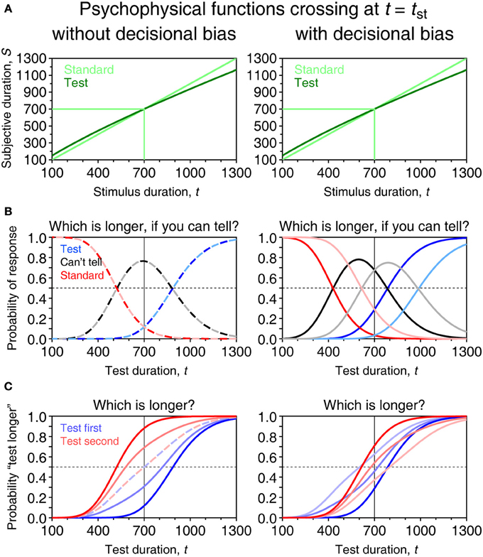
Figure 8. The PSE at the standard duration is not a sufficient condition for equality of time perception for test and standard stimuli. Graphical conventions and indifference regions for absence or presence of decisional bias as in Figure 7. (A) Different psychophysical functions for test and standard may cross at or very near t = tst. In this illustration, μs is the identity function whereas μt is given by Equation (1) with αt = 3.01, βt = 0.83, and τt = −10. As regards the scalar property in Equation (2), γs = 0.15 and γt = 0.10. (B) Psychometric functions in the ternary task, showing the signature of the PSE at t = tst = 700 ms regardless of the presence (left column) or absence (right column) of decisional bias and despite the different psychophysical functions for test and standard. (C) Psychometric functions for “test longer” responses in the comparative task, again showing the effects of decisional and response bias.
The foregoing discussion does not mean that adaptive methods should be entirely abandoned. On the contrary, some up–down methods provide dependable and efficient strategies for data collection and, thus, they gather maximally informative data for fitting psychometric functions. Adaptive methods tailored to the peculiarities of equality and ternary tasks have recently been developed (García-Pérez, 2014). For an illustration of their use, see García-Pérez and Peli (2014). What should be avoided by all means is the practice of estimating percent points by averaging reversal levels.
Pending Issues
It is unclear at this point whether the mathematical form of μ and σ in Equations (1)–(2) describe adequately the mean and standard deviation of subjective duration across the continuum from a few milliseconds to several seconds. Empirical studies suggest that a power function is adequate for μ within narrow time ranges but its parameters vary across ranges (Eisler, 1976), suggesting that a power function is only piecewise approximate. Although a yet unknown mathematical form might be more appropriate, the narrow range of durations used in any given study supports the use of Equation (1) on fitting psychometric functions. On the other hand, the scalar property in Equation (2) is known to be inaccurate in human timing but alternative mathematical forms have been proposed (Killeen et al., 1997; Rammsayer and Ulrich, 2001) that may prove more useful in practice. Also in this respect, it is unclear whether the referent for the scalar property is subjective time (as in Equation 2) or objective time.
Consideration of errors made by observers upon reporting judgments via the response interface has been intentionally excluded in this description. Extensions incorporating error parameters for more accurate parameter estimation have been discussed for analogous models elsewhere (García-Pérez and Alcalá-Quintana, 2012; García-Pérez and Peli, 2014) and their inclusion in the models presented here is straightforward.
Conflict of Interest Statement
The author declares that the research was conducted in the absence of any commercial or financial relationships that could be construed as a potential conflict of interest.
Acknowledgment
Supported by grant PSI2012-32903 from Ministerio de Economía y Competitividad (Spain).
References
Alcalá-Quintana, R., and García-Pérez, M. A. (2004). The role of parametric assumptions in adaptive Bayesian estimation. Psychol. Methods 9, 250–271. doi: 10.1037/1082-989X.9.2.250
Alcalá-Quintana, R., and García-Pérez, M. A. (2007). A comparison of fixed-step-size and Bayesian staircases for sensory threshold estimation. Spat. Vis. 20, 197–218. doi: 10.1163/156856807780421174
Alcalá-Quintana, R., and García-Pérez, M. A. (2011). A model for the time-order error in contrast discrimination. Q. J. Exp. Psychol. 64, 1221–1248. doi: 10.1080/17470218.2010.540018
Allan, L. G. (1983). Magnitude estimation of temporal intervals. Percept. Psychophys. 33, 29–42. doi: 10.3758/BF03205863
Allan, L. G. (2002a). The location and interpretation of the bisection point. Q. J. Exp. Psychol. 55B, 43–60. doi: 10.1080/02724990143000162
Allan, L. G. (2002b). Are the referents remembered in temporal bisection? Learn. Motiv. 33, 10–31. doi: 10.1006/lmot.2001.1097
Allan, L. G., and Gerhardt, K. (2001). Temporal bisection with trial referents. Percept. Psychophys. 63, 524–540. doi: 10.3758/BF03194418
Allman, M. J., and Meck, W. H. (2012). Patophysiological distortions in time perception and timed performance. Brain 135, 656–677. doi: 10.1093/brain/awr210
Allman, M. J., Teki, S., Griffiths, T. D., and Meck, W. H. (2014). Properties of the internal clock: first- and second-order principles of subjective time. Annu. Rev. Psychol. 65, 743–777. doi: 10.1146/annurev-psych-010213-115117
Angrilli, A., Cherubini, P., Pavese, A., and Manfredini, S. (1997). The influence of affective factors on time perception. Percept. Psychophys. 59, 972–982. doi: 10.3758/BF03205512
Arstila, V. (2012). Time slows down during accidents. Front. Psychol. 3:196. doi: 10.3389/fpsyg.2012.00196
Block, R. A. (1990). “Models of psychological time,” in Cognitive Models of Psychological Time, ed R. A. Block (Hillsdale, NJ: Erlbaum), 1–35.
Block, R. A., Zakay, D., and Hancock, P. A. (1999). Developmental changes in human duration judgments: a meta-analytic review. Dev. Rev. 19, 183–211. doi: 10.1006/drev.1998.0475
Campbell, L. A., and Bryant, R. A. (2007). How time flies: a study of novice skydivers. Behav. Res. Ther. 45, 1389–1392. doi: 10.1016/j.brat.2006.05.011
Carlson, V. R., and Feinberg, I. (1970). Time judgment as a function of method, practice, and sex. J. Exp. Psychol. 85, 171–180. doi: 10.1037/h0029504
Chen, L., and Vroomen, J. (2013). Intersensory binding across space and time: a tutorial review. Atten. Percept. Psychophys. 75, 790–811. doi: 10.3758/s13414-013-0475-4
Church, R. M., and Deluty, M. Z. (1977). Bisection of temporal intervals. J. Exp. Psychol. Anim. Behav. Process. 3, 216–228. doi: 10.1037/0097-7403.3.3.216
Church, R. M., and Gibbon, J. (1982). Temporal generalization. J. Exp. Psychol. Anim. Behav. Process. 8, 165–186. doi: 10.1037/0097-7403.8.2.165
Dawson, W. E., and Miller, M. E. (1978). Inverse attribute functions and the proposed modifications of the power law. Percept. Psychophys. 24, 457–465. doi: 10.3758/BF03199744
Dong, P., and Wyer, R. S. Jr. (2014). How time flies: the effects of conversation characteristics and partner attractiveness on duration judgments in a social interaction. J. Exp. Soc. Psychol. 50, 1–14. doi: 10.1016/j.jesp.2013.08.005
Droit-Volet, S. (2013). Time perception in children: a neurodevelopmental approach. Neuropsychologia 51, 220–234. doi: 10.1016/j.neuropsychologia.2012.09.023
Droit-Volet, S., and Izaute, M. (2009). Improving time discrimination in children and adults in a temporal bisection task: the effects of feedback and no forced choice on decision and memory processes. Q. J. Exp. Psychol. 62, 1173–1188. doi: 10.1080/17470210802384180
Dyjas, O., Bausenhart, K. M., and Ulrich, R. (2012). Trial-by-trial updating of an internal reference in discrimination tasks: evidence from effects of stimulus order and trial sequence. Atten. Percept. Psychophys. 74, 1819–1841. doi: 10.3758/s13414-012-0362-4
Dyjas, O., and Ulrich, R. (2014). Effects of stimulus order on discrimination processes in comparative and equality judgements: data and models. Q. J. Exp. Psychol. (Hove) 67, 1121–1150. doi: 10.1080/17470218.2013.847968
Eisler, A. D., and Eisler, H. (1994). Subjective time scaling: influence of age, gender, and type A and type B behavior. Chronobiologia 21, 185–200.
Eisler, H. (1976). Experiments on subjective duration 1868–1975: a collection of power function exponents. Psychol. Bull. 83, 1154–1171. doi: 10.1037/0033-2909.83.6.1154
Faes, F., Nollo, G., Ravelli, F., Ricci, L., Vescovi, M., Turatto, M., et al. (2007). Small-sample characterization of stochastic approximation staircases in forced-choice adaptive threshold estimation. Percept. Psychophys. 69, 254–262. doi: 10.3758/BF03193747
Fagot, R. F. (1975). A note on the form of the psychophysical function near threshold. Bull. Psychon. Soc. 6, 665–667. doi: 10.3758/BF03337601
Friedman, W. J., and Kemp, S. (1998). The effects of elapsed time and retrieval on young children's judgments of the temporal distances of past events. Cogn. Dev. 13, 335–367. doi: 10.1016/S0885-2014(98)90015-6
García-Pérez, M. A. (1998). Forced-choice staircases with fixed step sizes: asymptotic and small-sample properties. Vision Res. 38, 1861–1881. doi: 10.1016/S0042-6989(97)00340-4
García-Pérez, M. A. (2000). Optimal setups for forced-choice staircases with fixed step sizes. Spat. Vis. 13, 431–448. doi: 10.1163/156856800741306
García-Pérez, M. A. (2001). Yes-no staircases with fixed step sizes: psychometric properties and optimal setup. Optom. Vis. Sci. 78, 56–64. doi: 10.1097/00006324-200101010-00015
García-Pérez, M. A. (2002). Properties of some variants of adaptive staircases with fixed step sizes. Spat. Vis. 15, 303–321. doi: 10.1163/15685680260174056
García-Pérez, M. A. (2011). A cautionary note on the use of the adaptive up-down method. J. Acoust. Soc. Am. 130, 2098–2107. doi: 10.1121/1.3628334
García-Pérez, M. A. (2014). Adaptive psychophysical methods for nonmonotonic psychometric functions. Atten. Percept. Psychophys. 76, 621–641. doi: 10.3758/s13414-013-0574-2
García-Pérez, M. A., and Alcalá-Quintana, R. (2007a). The transducer model for contrast detection and discrimination: formal relations, implications, and an empirical test. Spat. Vis. 20, 5–43. doi: 10.1163/156856807779369724
García-Pérez, M. A., and Alcalá-Quintana, R. (2007b). Bayesian adaptive estimation of arbitrary points on a psychometric function. Br. J. Math. Stat. Psychol. 60, 147–174. doi: 10.1348/000711006X104596
García-Pérez, M. A., and Alcalá-Quintana, R. (2009a). Fixed vs. variable noise in 2AFC contrast discrimination: lessons from psychometric functions. Spat. Vis. 22, 273–300. doi: 10.1163/156856809788746309
García-Pérez, M. A., and Alcalá-Quintana, R. (2009b). Empirical performance of optimal Bayesian adaptive estimation. Span. J. Psychol. 12, 3–11. doi: 10.1017/S1138741600001426
García-Pérez, M. A., and Alcalá-Quintana, R. (2010a). Reminder and 2AFC tasks provide similar estimates of the difference limen: a reanalysis of data from Lapid, Ulrich, and Rammsayer (2008) and a discussion of Ulrich and Vorberg (2009). Atten. Percept. Psychophys. 72, 1155–1178. doi: 10.3758/APP.72.4.1155 [A correction was published: García-Pérez, M. A., and Alcalá-Quintana, R. (2012). Correction to “Reminder and 2AFC tasks provide similar estimates of the difference limen: a reanalysis of data from Lapid, Ulrich, and Rammsayer (2008) and a discussion of Ulrich and Vorberg (2009).” Atten. Percept. Psychophys. 74, 489–492. doi: 10.3758/s13414-012-0274-3]
García-Pérez, M. A., and Alcalá-Quintana, R. (2010b). The difference model with guessing explains interval bias in two-alternative forced-choice detection procedures. J. Sens. Stud. 25, 876–898. doi: 10.1111/j.1745-459X.2010.00310.x
García-Pérez, M. A., and Alcalá-Quintana, R. (2011a). Interval bias in 2AFC detection tasks: sorting out the artifacts. Atten. Percept. Psychophys. 73, 2332–2352. doi: 10.3758/s13414-011-0167-x
García-Pérez, M. A., and Alcalá-Quintana, R. (2011b). Improving the estimation of psychometric functions in 2AFC discrimination tasks. Front. Psychol. 2:96. doi: 10.3389/fpsyg.2011.00096
García-Pérez, M. A., and Alcalá-Quintana, R. (2012). On the discrepant results in synchrony judgment and temporal-order judgment tasks: a quantitative model. Psychon. Bull. Rev. 19, 820–846. doi: 10.3758/s13423-012-0278-y
García-Pérez, M. A., and Alcalá-Quintana, R. (2013). Shifts of the psychometric function: distinguishing bias from perceptual effects. Q. J. Exp. Psychol. 66, 319–337. doi: 10.1080/17470218.2012.708761
García-Pérez, M. A., and Peli, E. (2014). The bisection point across variants of the task. Atten. Percept. Psychophys. doi: 10.3758/s13414-014-0672-9. [Epub ahead of print].
Gava, L., Valenza, E., Di Bono, M. G., and Tosatto, C. (2012). Discrimination and ordinal judgments of temporal durations at 3 months. Infant Behav. Dev. 35, 751–760. doi: 10.1016/j.infbeh.2012.05.009
Gibbon, J. (1977). Scalar expectancy theory and Weber's law in animal timing. Psychol. Rev. 84, 279–325. doi: 10.1037/0033-295X.84.3.279
Gibbon, J. (1981). On the form and location of the psychometric bisection function for time. J. Math. Psychol. 24, 58–87. doi: 10.1016/0022-2496(81)90035-3
Gibbon, J. (1986). “The structure of subjective time: How time flies,” in The Psychology of Learning and Motivation, Vol. 20, ed G. H. Bower (London, UK: Academic Press), 105–135.
Gil, S., and Droit-Volet, S. (2011). “Time flies in the presence of angry faces”… depending on the temporal task used! Acta Psychol. 136, 354–362. doi: 10.1016/j.actpsy.2010.12.010
Gil, S., Rousset, S., and Droit-Volet, S. (2009). How liked and disliked foods affect time perception. Emotion 9, 457–463. doi: 10.1037/a0015751
Glicksohn, J., and Hadad, Y. (2012). Sex differences in time production revisited. J. Indiv. Dif. 33, 35–42. doi: 10.1027/1614-0001/a000059
Greenwald, A. G. (2012). There is nothing so theoretical as a good method. Perspect. Psychol. Sci. 7, 99–108. doi: 10.1177/1745691611434210
Grondin, S. (1998). Judgments of the duration of visually marked empty time intervals: linking perceived duration and sensitivity. Percept. Psychophys. 60, 319–330. doi: 10.3758/BF03206040
Grondin, S. (2010). Timing and time perception: a review of recent behavioral and neuroscience findings and theoretical directions. Atten. Percept. Psychophys. 72, 561–582. doi: 10.3758/APP.72.3.561
Grondin, S., and Rammsayer, T. (2003). Variable foreperiods and temporal discrimination. Q. J. Exp. Psychol. 56A, 731–765. doi: 10.1080/02724980244000611
Helson, H. (1948). Adaptation-level as a basis for a quantitative theory of frames of reference. Psychol. Rev. 55, 297–313. doi: 10.1037/h0056721
Hsu, Y.-F., and Chin, C.-L. (2014). On the limitations of fixed-step-size adaptive methods with response confidence. Br. J. Math. Stat. Psychol. 67, 266–283. doi: 10.1111/bmsp.12018
Kellaris, J. J., and Kent, R. J. (1992). The influence of music on consumers' temporal perceptions: does time fly when you're having fun? J. Consum. Psychol. 1, 365–376. doi: 10.1016/S1057-7408(08)80060-5
Killeen, P. R., Fetterman, J. G., and Bizo, L. A. (1997). “Time's causes,” in Time and Behaviour: Psychological and Neurobehavioural Analyses, eds C. M. Bradshaw and E. Szabadi (Amsterdam: Elsevier), 79–131. doi: 10.1016/S0166-4115(97)80055-6
Kopec, C. D., and Brody, C. D. (2010). Human performance on the temporal bisection task. Brain Cogn. 74, 262–272. doi: 10.1016/j.bandc.2010.08.006
Lewin, K. (1951). Field Theory in Social Science: Selected Theoretical Papers (Edited by D. Cartwright). New York, NY: Harper & Brothers.
Lewis, P. A., and Miall, R. C. (2009). The precision of temporal judgement: milliseconds, many minutes, and beyond. Philos. Trans. R. Soc. Lond. B Biol. Sci. 364, 1897–1905. doi: 10.1098/rstb.2009.0020
Magnotti, J. F., Ma, W. J., and Beauchamp, M. S. (2013). Causal inference of asynchronous audiovisual speech. Front. Psychol. 4:798. doi: 10.3389/fpsyg.2013.00798
Marks, L. E., and Stevens, J. C. (1968). The form of the psychophysical function near threshold. Percept. Psychophys. 4, 315–318. doi: 10.3758/BF03210523
Mioni, G., Stablum, F., McClintock, S. M., and Grondin, S. (2014). Different methods for reproducing time, different results. Atten. Percept. Psychophys. 76, 675–681. doi: 10.3758/s13414-014-0625-3
Misuraca, R., and Teuscher, U. (2013). Time flies when you maximize – Maximizers and satisficers perceive time differently when making decisions. Acta Psychol. 143, 176–180. doi: 10.1016/j.actpsy.2013.03.004
Ogden, R. S. (2013). The effect of facial attractiveness on temporal perception. Cogn. Emot. 27, 1292–1304. doi: 10.1080/02699931.2013.769426
Penney, T. B., Brown, G. D. A., and Wong, J. K. L. (2014). Stimulus spacing effects in duration perception are larger for auditory stimuli: data and a model. Acta Psychol. 147, 97–104. doi: 10.1016/j.actpsy.2013.07.017
Provasi, J., Rattat, A., and Droit-Volet, S. (2011). Temporal bisection in 4-month-old infants. J. Exp. Psychol. Anim. Behav. Process. 37, 108–113. doi: 10.1037/a0019976
Rammsayer, T., and Ulrich, R. (2001). Counting models of temporal discrimination. Psychon. Bull. Rev. 8, 270–277. doi: 10.3758/BF03196161
Raslear, T. G. (1985). Perceptual bias and response bias in temporal bisection. Percept. Psychophys. 38, 261–268. doi: 10.3758/BF03207153
Rattat, A.-C., and Droit-Volet, S. (2012). What is the best and easiest method of preventing counting in different temporal tasks? Behav. Res. Methods 44, 67–80. doi: 10.3758/s13428-011-0135-3
Rodríguez-Gironés, M. A., and Kacelnik, A. (2001). Relative importance of perceptual and mnemonic variance in human temporal bisection. Q. J. Exp. Psychol. 54A, 527–546. doi: 10.1080/713755980
Schneider, K. A., and Komlos, M. (2008). Attention biases decisions but does not alter appearance. J. Vis. 8, 3. doi: 10.1167/8.15.3
Simon, M. K. (2002). Probability Distributions Involving Gaussian Random Variables. New York, NY: Springer.
Spence, C., and Parise, C. (2010). Prior-entry: a review. Conscious. Cogn. 19, 364–379. doi: 10.1016/j.concog.2009.12.001
Tipples, J. (2010). Time flies when we read taboo words. Psychon. Bull. Rev. 17, 563–568. doi: 10.3758/PBR.17.4.563
Ulbrich, P., Churan, J., Fink, M., and Wittmann, M. (2007). Temporal reproduction: further evidence for two processes. Acta Psychol. 125, 51–65. doi: 10.1016/j.actpsy.2006.06.004
Ulrich, R., and Vorberg, D. (2009). Estimating the difference limen in 2AFC tasks: pitfalls and improved estimators. Atten. Percept. Psychophys. 71, 1219–1227. doi: 10.3758/APP.71.6.1219
Vroomen, J., and Keetels, M. (2010). Perception of intersensory synchrony: a tutorial review. Atten. Percept. Psychophys. 72, 871–884. doi: 10.3758/APP.72.4.871
Wackermann, J. (2011). “On clocks, models and metaphors: Understanding the Klepsydra model,” in Multidisciplinary Aspects of Time and Time Perception, eds A. Vatakis, A. Esposito, M. Giagkou, F. Cummins, and G. Papadelis (New York, NY: Springer), 246–257. doi: 10.1007/978-3-642-21478-3_19
Wearden, J. H. (1991a). Human performance on an analogue of an interval bisection task. Q. J. Exp. Psychol. 43B, 59–81.
Wearden, J. H. (1991b). Do humans possess an internal clock with scalar timing properties? Learn. Motiv. 22, 59–83. doi: 10.1016/0023-9690(91)90017-3
Wearden, J. H. (1992). Temporal generalization in humans. J. Exp. Psychol. Anim. Behav. Process. 18, 134–144. doi: 10.1037/0097-7403.18.2.134
Wearden, J. H., and Bray, S. (2001). Scalar timing without reference memory? Episodic temporal generalization and bisection in humans. Q. J. Exp. Psychol. 54B, 289–310. doi: 10.1080/02724990042000173
Wearden, J. H., and Ferrara, A. (1995). Stimulus spacing effects in temporal bisection by humans. Q. J. Exp. Psychol. 48B, 289–310. doi: 10.1080/14640749508401454
Wearden, J. H., and Ferrara, A. (1996). Stimulus range effects in temporal bisection by humans. Q. J. Exp. Psychol. 49B, 24–44. doi: 10.1080/713932615
Wearden, J. H., O'Rourke, S. C., Matchwick, C., Min, Z., and Maeers, S. (2010). Task switching and subjective duration. Q. J. Exp. Psychol. 63, 531–543. doi: 10.1080/17470210903024768
Keywords: perception of duration, psychophysical methods, psychophysical function, psychometric function, probabilistic models
Citation: García-Pérez MA (2014) Does time ever fly or slow down? The difficult interpretation of psychophysical data on time perception. Front. Hum. Neurosci. 8:415. doi: 10.3389/fnhum.2014.00415
Received: 04 March 2014; Accepted: 23 May 2014;
Published online: 10 June 2014.
Edited by:
José M. Medina, Universidad de Granada, SpainReviewed by:
Yoshitaka Nakajima, Kyushu University, JapanHannes Eisler, Stockholm University, Sweden
Copyright © 2014 García-Pérez. This is an open-access article distributed under the terms of the Creative Commons Attribution License (CC BY). The use, distribution or reproduction in other forums is permitted, provided the original author(s) or licensor are credited and that the original publication in this journal is cited, in accordance with accepted academic practice. No use, distribution or reproduction is permitted which does not comply with these terms.
*Correspondence: Miguel A. García-Pérez, Departamento de Metodología, Facultad de Psicología, Universidad Complutense, Campus de Somosaguas, Madrid 28223, Spain e-mail: miguel@psi.ucm.es