Modeling population spike trains with specified time-varying spike rates, trial-to-trial variability, and pairwise signal and noise correlations

Introduction

Correlated spiking activity in neuronal populations has been a subject of intense theoretical and experimental research over the past several decades, and the importance of correlations has been demonstrated in a number of contexts, including plasticity and information processing (for a recent review, see Averbeck et al., 2006). Recent advances in experimental technology have finally made it possible to observe the activity of large neuronal populations simultaneously. In order to take full advantage of these advances, new methods for the analysis and modeling of population activity must also be developed.

A number of methods exist for modeling correlated population spike trains in which some fraction of the input driving the activity of each neuron is shared with other neurons, including integrate-and-fire models and other spiking models with correlated input currents or synaptic conductances (Destexhe and Pare, 1999; Feng and Brown, 2000; Song and Abbott, 2001; Stroeve and Gilen, 2001; Salinas and Sejnowski, 2002; Dorn and Ringach, 2003; Gutig et al., 2003; Galan et al., 2006; De La Rocha et al., 2007; Shea-Brown et al., 2008; Tchumatchenko et al., 2008), stochastic spiking models with correlated rate functions (Galan et al., 2006; Brette, 2009; Krumin and Shoham, 2009), and models based on a dichotomized Gaussian (DG) framework (Macke et al., 2009; Gutnisky and Josic, 2010). There are also a variety of methods for capturing precise synchrony between neurons through explicit sharing of spikes (Kuhn et al., 2003; Galan et al., 2006; Niebur, 2007; Brette, 2009) and several models based on statistical frameworks such as maximum entropy (Schneidman et al., 2006; Shlens et al., 2006; Roudi et al., 2009).

All of the approaches described above are designed to capture and/or control the total correlation between spike trains and, as such, are of limited utility in the context of early sensory systems where it is important to separate internal network correlations from those due to the external stimulus. In this paper, we propose a framework designed specifically to model spike trains in which the total correlation can be separated into signal and noise components. If responses to repeated trials of an identical sensory stimulus are observed, the signal correlation, which reflects both correlation in the stimulus itself and similarities in neurons’ preferred stimulus features, will be evident in the fraction of the response that is repeatable from trial-to-trial. Noise correlation, which results from the activity of network and intrinsic cellular mechanisms, will be evident in the fraction of the response that is variable from trial-to-trial (note that the term noise correlation is not meant to imply that the activity underlying this correlation is unimportant, but simply that is not directly dependent on the stimulus).

For modeling the population spike trains of early sensory neurons, another class of methods based on generalized linear models (GLMs) has been developed (Chornoboy et al., 1988; Paninski, 2004; Kulkarni and Paninski, 2007; Paninski et al., 2007; Pillow et al., 2008). In its typical formulation, the GLM is parameterized by a series of filters that relate the time-varying spike rate in one neuron to the sensory stimulus and the responses of other neurons. This formulation has the great strength that once the filter parameters have been estimated, the model can be used not only to simulate responses that match those measured experimentally, but also to simulate responses to novel stimuli. However, this generality comes at a cost: specifying the filters requires the estimation of a large number of parameters and, thus, a large amount of experimental data – much more than is necessary for a model designed only to simulate responses to the same stimuli that have been tested experimentally. It is possible to formulate alternatives to the typical GLM that require less experimental data by forgoing the ability to predict responses to novel stimuli and parameterizing the time-varying firing rate in response to a particular stimulus directly. However, even in this formulation, the GLM lacks a critical property: it does not enable straightforward specification or manipulation of one response property independent of the others (Krumin and Shoham, 2009; Toyoizumi et al., 2009).

In the model we present below, the time-varying spike rate, trial-to-trial variability, and pairwise signal and noise correlations can be matched to those measured experimentally, and the noise correlations can be manipulated without changes in the signal correlations or the single-cell properties. The model is an extension of previous attempts to model population spike trains as DGs (Emrich and Piedmonte, 1991; Cox and Wermuth, 2002; Macke et al., 2009; Gutnisky and Josic, 2010). In our model, the response of each cell is a binary vector determined by the thresholded sum of two inputs: a signal, which is the same for each trial of a given stimulus, and a noise, which is different for each trial, both of which can be correlated across neurons. In the first part of the paper, we show how the model parameters can be estimated from experimental data and used to simulate spike trains with properties that match those measured experimentally. We also demonstrate how the model parameters can be manipulated to obtain spike trains with arbitrary pairwise noise correlations without changes in single-cell properties. In the second part of the paper, we describe a general form of the model that can be used model spike trains with arbitrary single-cell properties and pairwise correlations.

All of the Matlab code required to perform the analyses described in this paper is available for download at http://www.ucl.ac.uk/ear/research/lesicalab.

A Model for Simulating and Manipulating Experimentally Recorded Population Spike Trains

Single-Cell Responses

To represent a set of spike times from a single cell on a single trial i ∈ {1, 2,…,I} of a particular stimulus, we discretize time into n ∈ {1, 2,…,N} bins of length Δ and set r_i[n] = 1 if a spike occurs in bin n on trial i, and r_i[n] = 0 otherwise. In general, we assume that Δ is small enough that no more than one spike occurs in any given bin. Based on the responses to all trials r (an N × I binary matrix), we can define several quantities of interest:

Note that we use the notation 〈·〉_x to represent the expectation over all possible values of x, 〈·〉_x,y to represent the expectation over all possible values of x followed by the expectation of all possible values of y, and 〈·〉_x≠y to represent the expectation over all possible combinations of x and y in which their values are not equal. We chose to use the above definition of SNR as the measure of trial-to-trial variability because is it commonly used in early sensory systems (Borst and Theunissen, 1999). One important property of this measure that should be noted is that its value is dependent on the bin size Δ. Thus, all of the computations described below for fitting model parameters must be repeated if the bin size is changed.

We model the response as a dichotomized sum of a deterministic “signal” and Gaussian “noise”

Where r_i[n] is the response in time bin N on trial i, s (an N-dimensional vector) is the same on every trial and (an N-dimensional vector) is different on every trial [note that neither s nor z are intended to correspond directly to any intracellular quantities]. Given the experimentally recorded responses of a cell, we wish to simulate responses with the same PSTH This can be done by solving

for s[n] in each bin, where Φ(x, σ²) is the CDF for a Gaussian with zero mean and variance σ² evaluated at x. Equation 2 is easily solved numerically, as the function is monotonic and has unique level crossings. It is clear from Eq. 2 that the choice of one for the variance of z is somewhat arbitrary; for any finite value of the variance of z, an s[n] can be found to achieve any desired value of Note that if then s[n] must be either −∞ or +∞. If finite values of s[n] are desired, then can be constrained to the interval [1/I, 1 − 1/I] before solving Eq. 2.

Importantly, since this approach matches exactly, it will also match the mean spike probability r₀ and the spike train signal to noise ratio SNR, as both can be uniquely defined in terms of the PSTH

where, because r_i is binary,

Matching exactly will also match the mutual information transmitted by single spikes (Brenner et al., 2000). Note that if it is not necessary to match the bin to bin spike probabilities of the experimental response, but only the distribution of overall spike counts, a reduced model can be used (Macke et al., 2009).

To demonstrate the utility of this model, we first generated responses using Eq. 1 with a variety of different signals, and then attempted to reproduce the model responses after estimating s using Eq. 2. Typical results are shown in Figure 1A. For uniform random, sine wave, and square wave signals, the PSTH and, consequently, r₀ and SNR of the responses simulated with the estimated s closely match those of the original model generated data.

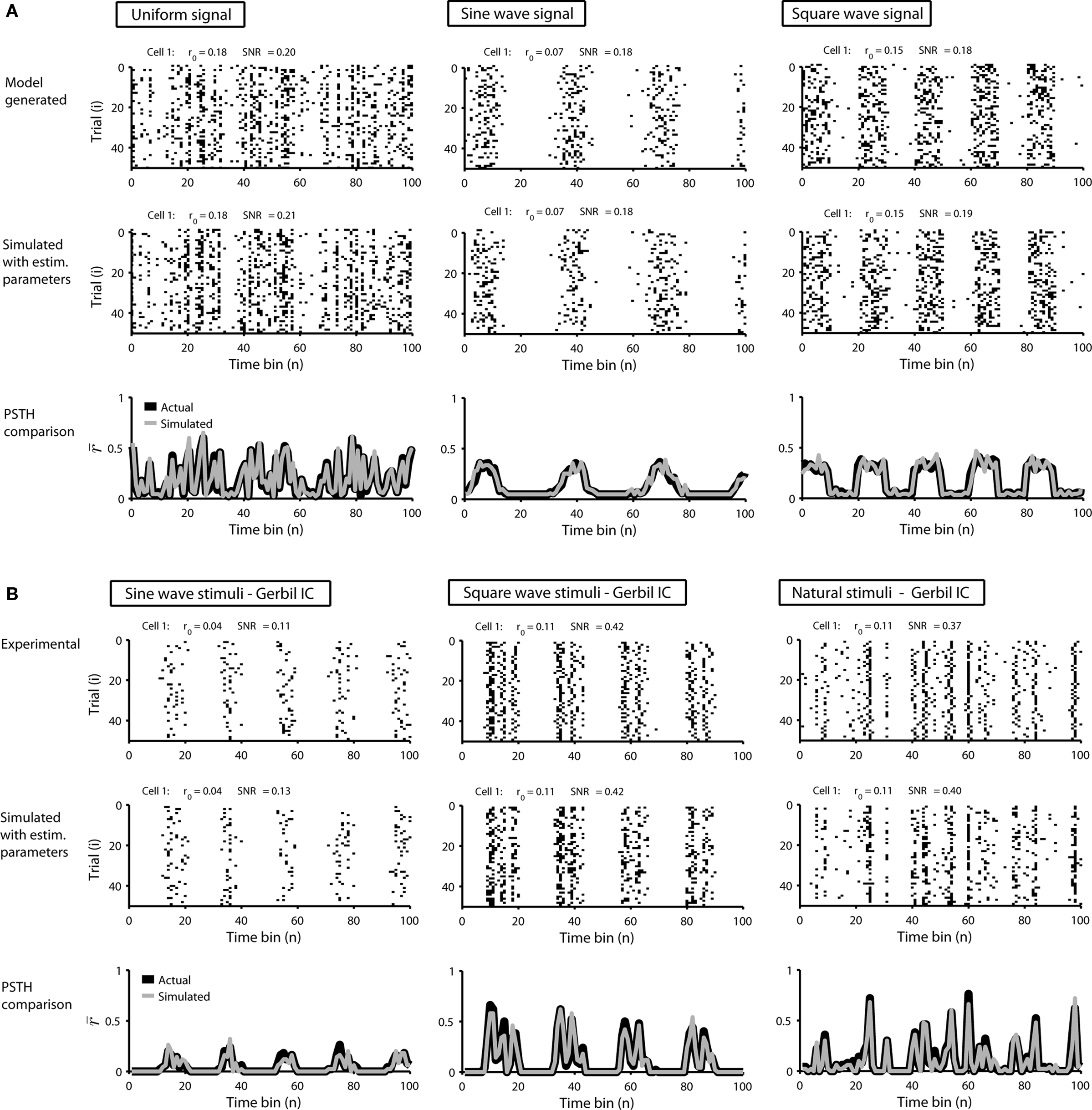
Figure 1. Simulated responses match the single-cell properties of model generated and experimental data. (A) The top row shows model generated responses to repeated trials with a variety of waveforms for s: a uniform random noise signal in the range [−0.5 to 0.5]; a sinusoidal signal 0.75 sin(n/5) − 1; a square wave signal with a 50% duty cycle, a period of 20 samples, and the same mean value and peak-to-peak amplitude as the sinusoid. The middle row shows simulated responses with s estimated from the responses in the top row. The bottom row shows the PSTHs of the original model generated (black) and simulated (gray) responses. (B) The top row shows experimental responses of a cell recorded in the inferior colliculus of an anesthetized gerbil to repeated trials of a variety of sounds (experimental methods are described in Lesica and Grothe, 2008a,b): a sinusoidally amplitude modulated (SAM) tone with a carrier frequency of 6 KHz, a modulation depth of 100%, an intensity of 70 dB, and a modulation frequency of 50 Hz; a square wave modulated tone with the same carrier frequency, modulation depth, and intensity, a 50% duty cycle, and a period of 25 ms; a tone with the same carrier frequency and intensity modulated by a signal with power spectra matched to that measured from a series of animal vocalizations. The bin size Δ for these responses was 1 ms. The middle and bottom rows show the simulated responses simulated and PSTHs presented as in (A).

Next, we tested the model’s ability to reproduce the single-cell properties of experimentally recorded responses. Figure 1B shows the responses of neurons in the gerbil inferior colliculus to repeated presentations of a variety of sounds. In each case, we estimated s from the experimental data using Eq. 2 and were able to simulate new responses with PSTH, r₀, and SNR that match those measured experimentally.

Population Responses

As described in the Introduction, correlations between cells in early sensory systems can have both signal and noise components: signal correlations arise from correlations in the stimulus itself and/or similarity in preferred stimulus features (frequency, orientation, etc.), while noise correlations arise from shared inputs that contribute to the trial-to-trial variability in responses. In our model, we adopt the most common definition of noise correlation, where the noise correlation between cells p and q, is given by the difference between the total correlation and the signal correlation, and and are the correlation coefficients between the responses of cells p and q before and after the trial order has been shuffled. The model described above for a single cell is easily extended to capture the pairwise signal and noise correlations in a population, where the response of cell p ∈ {1, 2,…,P} is given by

where each cell has its own s^p that is the same on every trial and z^p that is different on every trial. In this population model, z ∼ 𝒩(0, σ_z) is a multivariate (P-dimensional) Gaussian random process with covariance matrix

where which is assumed to be constant across time bins and trials, is the pairwise correlation coefficient between z^p and z^q and Assuming we have the responses of a population to repeated trials of a particular stimulus, we can estimate each s^p separately to match the single-cell properties as described above. Because the response is binary and this approach matches exactly for each cell, it will also match the signal correlation between cells. To match the noise correlation, it is necessary to find the appropriate covariance matrix σ_z. This can be done by solving the equation that relates to the spike train noise correlation numerically for each pair of cells (again, the function is monotonic and, because z is Gaussian, each can be solved for independently).

Thus, can be written as

where, because r_i is binary,

and, because z is Gaussian,

where is the CDF for a two-dimensional Gaussian with zero mean and covariance ∑ evaluated at

To demonstrate the utility of this approach, we first attempted to reproduce the single-cell properties and pairwise correlations recorded experimentally from a population of 10 cells in the cat lateral geniculate nucleus in response to repeated presentations of a natural scene movie. Figure 2A shows the experimental and simulated responses for two cells. As expected, the PSTH, r₀, and SNR of the experimental and simulated responses are closely matched. As shown in Figure 2B, the measured and simulated pairwise noise correlations in the population are also closely matched.

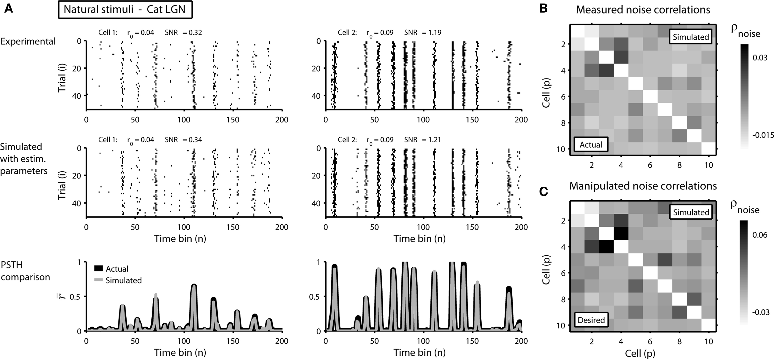
Figure 2. Simulated responses match the single-cell properties and pairwise correlations in experimental data. (A) The top row shows the experimental responses of two cells recorded simultaneously in the lateral geniculate nucleus of an anesthetized cat to repeated trials of a natural scene movie (experimental methods are described in Lesica et al., 2007) with an RMS contrast of 0.4. The bin size Δ for these responses was 4 ms. The middle and bottom rows show the simulated responses and PSTHs presented as in Figure 1. (B) The image shows the pairwise noise correlations in the experimental (lower triangular portion) and simulated (upper triangular portion) responses of a population of 10 neurons recorded in the cat LGN. The responses of all 10 cells were recorded simultaneously. (C) The image shows the desired pairwise noise correlations (lower triangular portion; values are double those measured in the original data) and the pairwise noise correlations realized in the simulated responses (upper triangular portion).

In addition to matching the experimentally observed responses, this approach can also be used to manipulate pairwise correlations without disturbing single-cell properties by changing the value of on the left side of Eq. 4 before solving for (note that there are a number of constraints on the realizable values of – for example, because the covariance matrix σ_z must be positive semi-definite, it may be difficult to obtain strong negative correlations; see Macke et al., 2009 for a detailed discussion). As a demonstration, we attempted to simulate population spike trains in which the noise correlations were twice as large as those observed experimentally. As shown in Figure 2C, the noise correlations in the simulated data match those desired.

Evaluating Goodness of Fit

Our model is not fit directly to observed spike trains, but rather to the PSTHs and pairwise noise correlations that are extracted from them. In our framework, any set of PSTHs and noise correlations can be fit with a unique set of model parameters, but that does not mean, of course, that the model is a good description of the original spike trains. The actual goodness of fit of the model is determined by two factors: the measurement noise in the PSTHs and noise correlations and the validity of the assumption that the spike trains can be described by our model framework. The goodness of fit can be measured by separating the available spike trains into “training” and “testing” sets, fitting the model parameters on the training spike trains, and calculating the (log) likelihood of the testing spike trains from the resulting model. The absolute likelihood may be difficult to interpret, but the ratio of the likelihoods from two different models can give be an informative measure.

To demonstrate the use of likelihood as a measure of goodness of fit, we simulated population spike trains from a known model (see figure legend for model parameters), split the spike trains into training and testing sets, and estimated the model parameters from the training spike trains. To determine whether including noise correlations in the estimated model improved the goodness of fit, we then compared the likelihood of the testing spike trains from the estimated model with and without noise correlations (i.e., with ∑_z estimated as described above or set to the identity matrix) for different numbers of training trials. The likelihood of a given testing spike train was computed as

where r_i is the N × P binary matrix of the responses of a population of P cells on a given trial i, r_i[n] is the vector of the responses for each cell, s[n] is the vector of the signals s^p[n] for each cell, is the CDF for a P-dimensional Gaussian with zero mean and covariance ∑ evaluated at and · denotes a point-by-point vector product. To isolate the effects of the noise correlations on the goodness of fit, we set the PSTHs in the estimated model to be the same as those in the actual model and used only the estimated noise correlations. As shown in Figure 3, as the number of training trials increased, the measurement noise in noise correlations decreased, and the likelihood from the estimated model with noise correlations approached that of the actual model, reaching the same value with I = 80 trials.

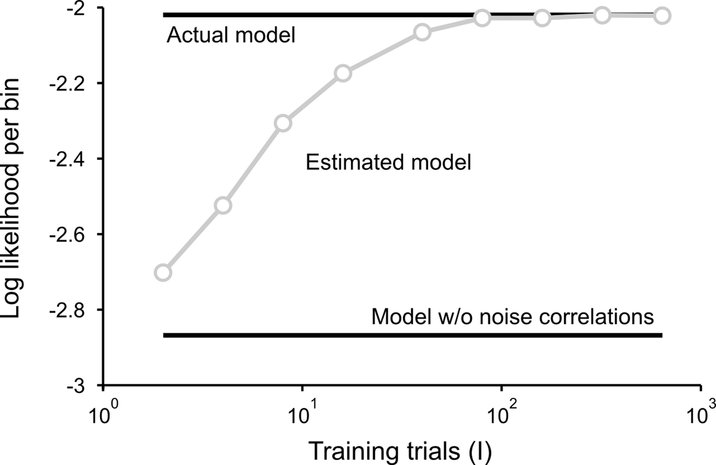
Figure 3. Model goodness of fit increases with increasing trials. The gray circles show the log likelihood (per bin) for the estimated model as a function of the number of trials used for fitting Σ_z. The likelihood was computed for 100 trials not used for fitting the model. The likelihoods for the actual model with and without noise correlations are also shown. Spike trains were generated using the model described in Eq. 10 with the following parameters: N = 500, P = 10, and θ were chosen so that r₀ ∼ 𝒩(0.16, 0.04) and SNR ∼ 𝒩(0.5, 0.35), and and were chosen so that and

Noise with Temporal Correlations

The model as described above captures both the instantaneous and long-term signal correlations between cells by matching their individual PSTHs, but captures only instantaneous noise correlations because z is uncorrelated in time. While instantaneous noise correlations are likely to be sufficient to describe population spike trains in early sensory systems, the model can also be extended to capture long-term noise correlations if necessary, for example, to capture the high level of trial-to-trial variability in higher cortical areas. Long-term noise correlations can be captured by adding temporal correlations to z via Gaussian conditioning (MacKay, 2003; Macke et al., 2009) so that z in each time bin is drawn from a distribution with mean and covariance dependent on the values of z in the preceding time bins:

and K is the number of preceding time bins to condition on. An example of such conditioning is shown in Figure 4. We used a known model to generate population spike trains with the noise auto- and cross-correlation functions shown by the thick black lines (see figure legend for model parameters). We then estimated model parameters from those spike trains, including those required for conditioning z on the preceding K = 4 time bins. The noise auto- and cross-correlation functions for the spike trains simulated from the estimated model (shown by the gray circles) closely match those of the original spike trains.

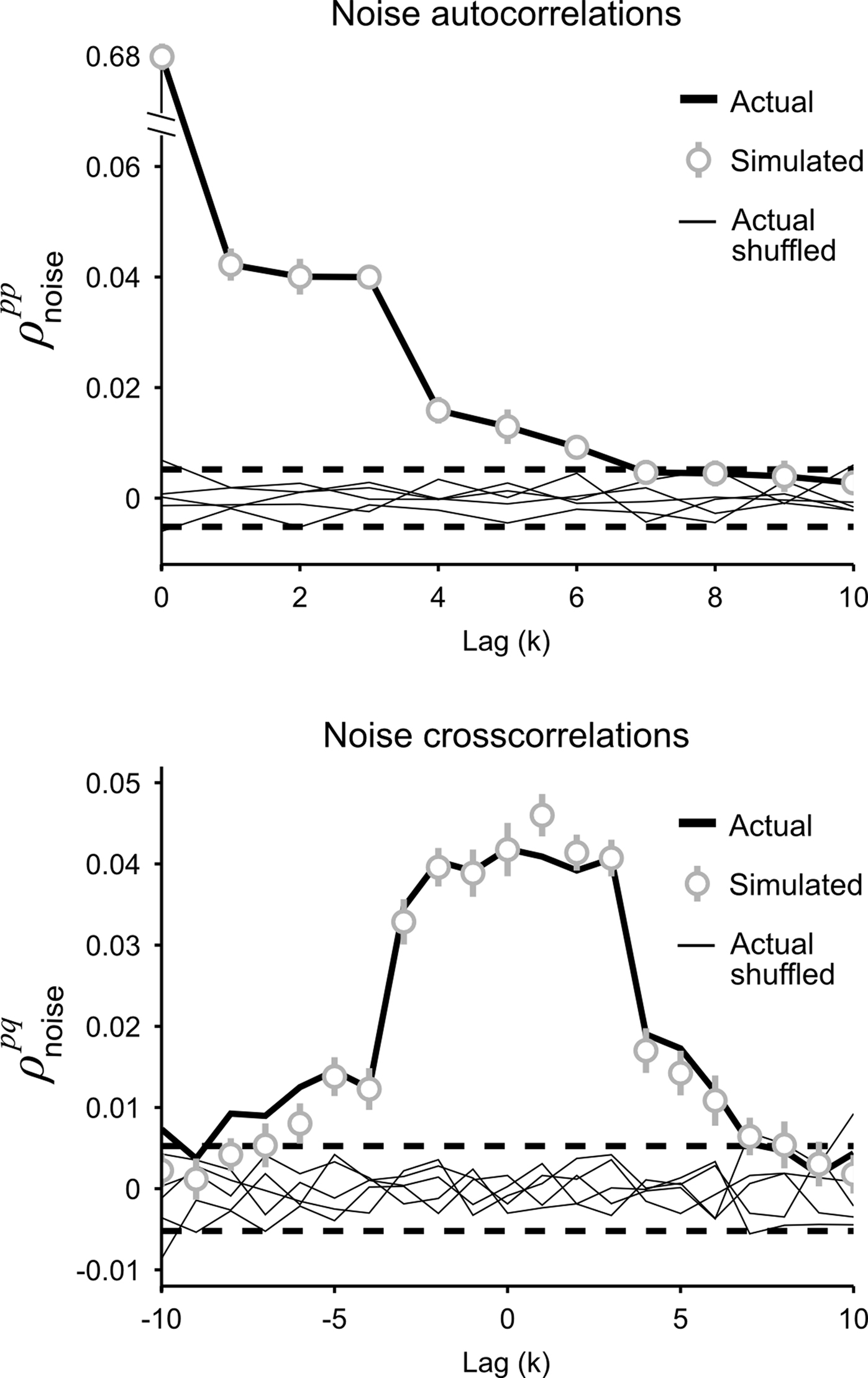
Figure 4. Gaussian conditioning captures long-term noise correlations. The gray circles show the noise auto- and cross-correlation functions for spike trains simulated from the estimated model. Error bars represent the standard deviation in the correlation values computed from independent realizations of the model. The model parameters were estimated from spike trains simulated by the model in Eq. 10, including Gaussian conditioning of z, with the following parameters: N = 500, P = 10, and θ were chosen so that r₀ ∼ 𝒩(0.16, 0.04) and SNR ∼ 𝒩(0.5, 0.35), and and for k ≤ 4 and zero thereafter. The noise auto- and cross-correlation functions of the original spike trains are shown by the thick black lines. Examples of the noise auto- and cross-correlation functions of the original spike trains after trial shuffling are shown by the thin black lines. The dashed lines indicate the mean ±2 standard deviations of the distribution of the correlation values after shuffling.

A General Model for Population Spike Trains

Single-Cell Responses

When modeling experimental spike trains as described above, the noise correlations can be chosen arbitrarily, but the mean spike rate, trial-to-trial variability, and signal correlations are dependent on the PSTH. It may also be useful to have a general model for population spike trains in which all of the response properties can be specified independently. For a single cell, this is achieved by replacing the deterministic signal s in the model framework described above with a Gaussian random process:

where is again a Gaussian random process that is different on every trial, s is a Gaussian random process that is the same on every trial, and the threshold θ is allowed to take on any value (note that in this case, θ cannot simply be set to an arbitrary value; in order to achieve any combination of r₀ and SNR, 2 degrees of freedom are required). Such a model could be used, for example, to simulate spike trains with any mean spike rate and trial-to-trial variability. Furthermore, because the model is based on Gaussian processes, it may enable certain population response properties to be investigated analytically or numerically directly from the model parameters, without the need for simulations.

To specify the model parameters, the equations for r₀ and SNR can be written in terms of and θ and solved numerically to obtain the appropriate values:

While Eq. 8 is already written in terms of and θ, Eq. 9 requires some manipulation. The numerator can be written as

where, because r_i is binary,

and, because s and z are Gaussian,

The denominator can be written as

where, because r_i is binary and s and z are Gaussian,

Note that in these equations, and r_i·r_j denotes point-by-point vector products, and denotes point-by-point squaring. Thus, for any realizable combination of r₀ and SNR, appropriate and θ can be found (the minimum realizable SNR depends on the number of trials, see Appendix). To demonstrate this approach, we randomly chose a variety of values for r₀ and SNR, estimated the corresponding values of and θ, and generated responses using the estimated values. As shown in Figure 5A, r₀ and SNR of the simulated responses closely match the desired values.

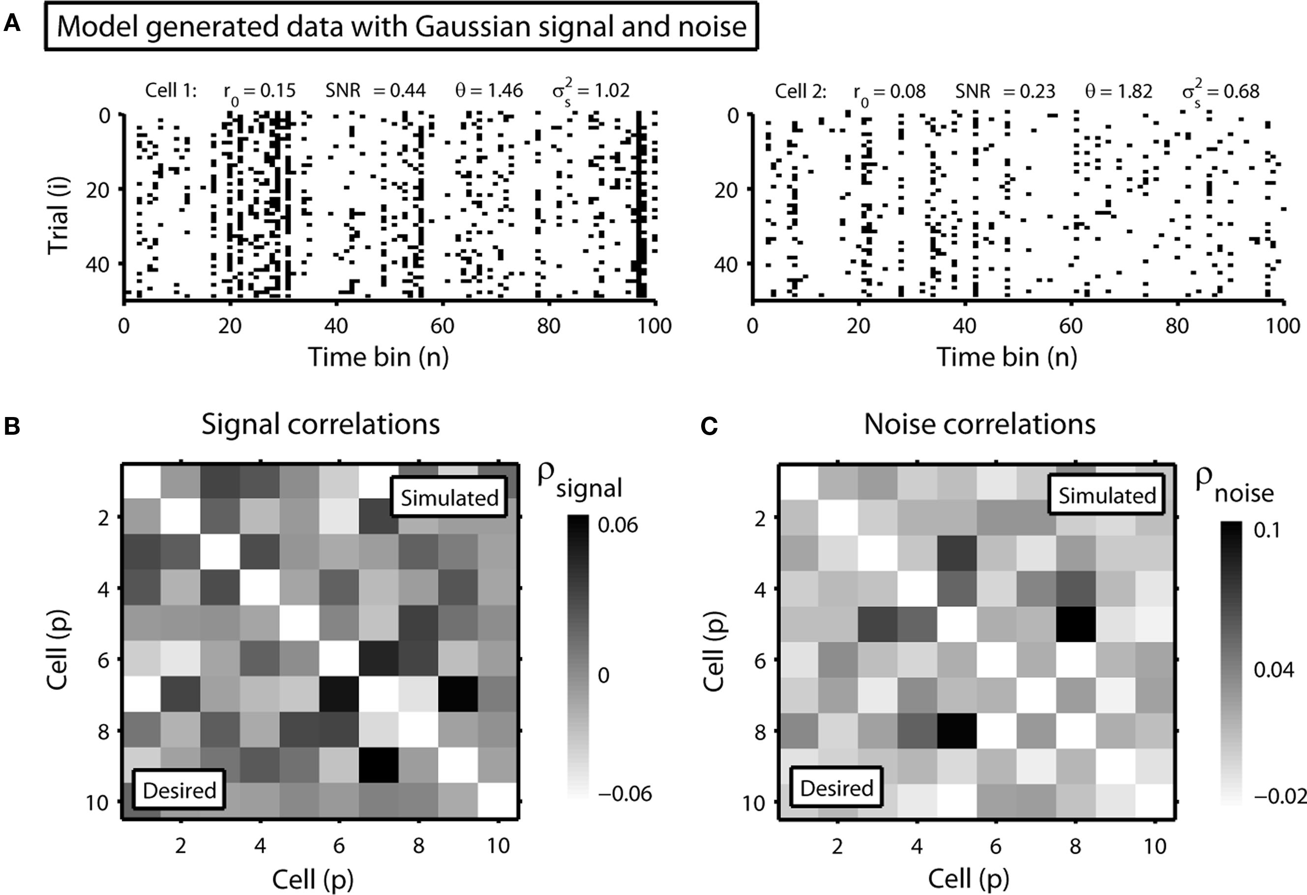
Figure 5. Simulated population responses with specified single-cell properties and pairwise correlations. (A) The top row shows the simulated responses for two cells with specified r₀ and SNR. (B) The image shows the desired pairwise signal correlations (lower triangular portion) and the pairwise signal correlations realized in the simulated responses (upper triangular portion) for a population of 10 cells. (C) The desired and realized pairwise noise correlations for a population of 10 cells presented as in (B).

Population Responses

The model described above for a single cell is easily extended to a population, where the response of cell p ∈ {1, 2,…,P} is given by

where both s and z are multivariate Gaussian random process s ∼ 𝒩(0, σ_s) and z ∼ 𝒩(0, ∑_z) with covariance matrices

After determining and θ for each cell based on the desired r₀ and SNR as described above, the pairwise correlation coefficients and required to obtain the desired spike train signal and noise correlations and can be found by solving the following equations numerically:

where, because r_i is binary,

and, because s and z are Gaussian,

Again, the functions are monotonic and each and can be solved for independently.

To demonstrate this approach, we generated a random set of pairwise signal and noise correlation coefficients and estimated the corresponding values of and and simulated population spike trains with these values. As shown in Figures 5B,C, the correlations in the simulated spike trains closely matched the desired values.

Discussion

We have described a model for simulating population spike trains typical of early sensory systems. The model has two forms: the first requires the specification of PSTHs and noise correlations and can be used to match and manipulate experimental data, and the second is more general and allows for population spike trains with any mean spike rates, trial-to-trial variabilities, signal correlations, and noise correlations. Both forms of the model are easily implemented as parameter fitting requires simply finding the level crossings of monotonic functions and correlations can be determined independently for each pair of cells. The Matlab code required to fit the model parameters is available for download at http://www.ucl.ac.uk/ear/research/lesicalab.

Our model improves on the existing methods for generating population spike trains described in the Introduction in several important ways. First, the model framework is explicitly designed around the response properties that are important for early sensory neurons: time-varying spike rate (PSTH), trial-to-trial variability, and signal and noise correlations. Second, the model allows independent and straightforward manipulation of one response property without changes in the other properties. One can imagine a number of potential uses for a model with these properties. The fact that the model matches the single-cell properties and correlations observed experimentally is in itself of some utility, such as providing a simple framework for computing the likelihood of observed spike trains given only pairwise interactions. These likelihoods could be used to, for example, test how important noise correlations are in determining population spike patterns by comparing models with and without noise correlations. The model also provides the ability to manipulate noise correlations without affecting the signal correlations or single-cell properties. In the brain, these properties are coupled to each other – for example, one can decrease the spike rate of visual neurons by decreasing the contrast of the stimulus, but this will also likely change the trial-to-trial variability and the correlations. Thus, a question such as whether or not changes in correlations with changes in contrast are detrimental or beneficial to a population code is impossible to answer experimentally. With our model, one could compare simulated populations with high contrast single-cell properties and correlations to simulated populations with high contrast single-cell properties and low contrast correlations to directly test whether or not the change in correlations is important. A similar example can be used to illustrate the utility of the general form of the model: Because the general form of the model allows for spike trains with any mean spike rate, trial-to-trial variability, and pairwise signal and noise correlations (within statistical constraints), it could be used to perform a systematic investigation of the effects of noise correlations on populations with different levels of signal correlations that would be impossible to conduct experimentally.

There are several ways in which the formulation of our model described here could potentially be improved. For example, the assumption that no more than one spike can occur in any time bin could potentially be relaxed, using a formulation analogous to that described in (Macke et al., 2009). Also, the current formulation of the model cannot be directly connected to biophysical quantities, so its parameters cannot be used, for example, to determine the current necessary to achieve a desired set of correlations in a stimulation experiment. With further effort, however, it may be possible to extend some of the desirable properties of our model into a more realistic framework such as an integrate-and-fire model (Paninski et al., 2004). Another limitation of the model that may be difficult to overcome is that in estimating a single value for each parameter across all trials, it implicitly assumes that the population is stationary. Certain types of non-stationarities, such as trial-to-trial fluctuations in the PSTH, may be captured by introducing long-term noise correlations via Gaussian conditioning, but others may require integrating the model into an adaptive framework (Eden et al., 2004).

There are also certain limitations of the model that are inherent in its underlying statistical framework. For example, it is difficult to generate spike trains with very low SNRs with a small number of trials – even if the variance of the internal signal in the model because the spikes are generated stochastically, the PSTH computed from a small number of trials will not have zero variance, and, thus, the SNR will not be zero. There are also constraints on the values of signal and noise correlations that can be achieved. Because the model is based on multivariate Gaussian processes which must have positive semi-definite covariance matrices, it is difficult, for example, to generate spike trains with strong negative correlations. Finally, while the model can be specified and fit to a population of any size, it is only guaranteed to capture second-order correlations. As with any model that includes only pairwise interactions, our model’s ability to capture the higher-order structure in population spike trains will depend on the nature of the population (Schneidman et al., 2006; Shlens et al., 2006; Roudi et al., 2009; Ohiorhenuan et al., 2010).

Conflict of Interest Statement

The authors declare that the research was conducted in the absence of any commercial or financial relationships that could be construed as a potential conflict of interest.

Acknowledgments

We thank Benedikt Grothe for the use of the gerbil data and Chong Weng, Jianzhong Jin, Chun-I Yeh, Dan Butts, Garrett Stanley, and Jose-Manuel Alonso for the use of the cat data. Dmitry R. Lyamzin and Nicholas A. Lesica were supported by the Deutsche Forschungsgemeinschaft (LE2522/1-1) and the Wellcome Trust. Jakob H. Macke was supported by the German Ministry of Education, Science, Research and Technology through the Bernstein award to Matthias Bethge (BMBF; FKZ: 01GQ0601).

References

Averbeck, B. B., Latham, P. E., and Pouget, A. (2006). Neural correlations, population coding and computation. Nat. Rev. Neurosci. 7, 358–366.
Borst, A., and Theunissen, F. E. (1999). Information theory and neural coding. Nat. Neurosci. 2, 947–957.
Brenner, N., Strong, S. P., Koberle, R., Bialek, W., de Ruyter van Steveninck, R. R. (2000). Synergy in a neural code. Neural Comput. 12, 1531–1552.
Chornoboy, E., Schramm, L., and Karr, A. (1988). Maximum likelihood identification of neural point process systems. Biol. Cybern. 59, 265–275.
Cox, D. R., and Wermuth, N. (2002). On some models for multivariate binary variables parallel in complexity with the multivariate Gaussian distribution. Biometrika 89, 462–469.
De La Rocha, J., Doiron, B., Shea-Brown, E., Josić, K., and Reyes, A. (2007). Correlation between neural spike trains increases with firing rate. Nature 448, 802–806.
Destexhe, A., and Pare, D. (1999). Impact of network activity on the integrative properties of neocortical pyramidal neurons in vivo. J. Neurophysiol. 81, 1531.
Dorn, J. D., and Ringach, D. L. (2003). Estimating membrane voltage correlations from extracellular spike trains. J. Neurophysiol. 89, 2271–2278.
Eden, U. T., Frank, L. M., Barbieri, R., Solo, V., and Brown, E. N. (2004). Dynamic analysis of neural encoding by point process adaptive filtering. Neural Comput. 16, 971–998.
Emrich, L. J., and Piedmonte, M. R. (1991). A method for generating high-dimensional multivariate binary variates. Am. Stat. 45, 302–304.
Feng, J., and Brown, D. (2000). Impact of correlated inputs on the output of the integrate-and-fire model. Neural Comput. 12, 671–692.
Galan, R. F., Fourcaud-Trocme, N., Ermentrout, G. B., and Urban, N. N. (2006). Correlation-induced synchronization of oscillations in olfactory bulb neurons. J. Neurosci. 26, 3646.
Gutig, R., Aharonov, R., Rotter, S., and Sompolinsky, H. (2003). Learning input correlations through nonlinear temporally asymmetric Hebbian plasticity. J. Neurosci. 23, 3697.
Gutnisky, D. A., and Josic, K. (2010). Generation of spatiotemporally correlated spike trains and local field potentials using a multivariate autoregressive process. J. Neurophysiol. 103, 2912–2930.
Krumin, M., and Shoham, S. (2009). Generation of spike trains with controlled auto-and cross-correlation functions. Neural Comput. 21, 1642–1664.
Kuhn, A., Aertsen, A., and Rotter, S. (2003). Higher-order statistics of input ensembles and the response of simple model neurons. Neural Comput. 15, 67–101.
Kulkarni, J. E., and Paninski, L. (2007). Common-input models for multiple neural spike-train data. Network 18, 375–407.
Lesica, N. A., and Grothe, B. (2008a). Efficient temporal processing of naturalistic sounds. PLoS ONE 3, e1655. doi: 10.1371/journal.pone.0001655.
Lesica, N. A., and Grothe, B. (2008b). Dynamic spectrotemporal feature selectivity in the auditory midbrain. J. Neurosci. 28, 5412–5421.
Lesica, N. A., Jin, J., Weng, C., Yeh, C. I., Butts, D. A., Stanley, G. B., and Alonso, J. M. (2007). Adaptation to stimulus contrast and correlations during natural visual stimulation. Neuron 55, 479–491.
MacKay, D. J. C. (2003). Information Theory, Inference, and Learning Algorithms. Cambridge: Cambridge University Press.
Macke, J. H., Berens, P., Ecker, A. S., Tolias, A. S., and Bethge, M. (2009). Generating spike trains with specified correlation coefficients. Neural Comput. 21, 397–423.
Niebur, E. (2007). Generation of synthetic spike trains with defined pairwise correlations. Neural Comput. 19, 1720–1738.
Ohiorhenuan, I. E., Mechler, F., Purpura, K. P., Schmid, A. M., Hu, Q., and Victor, J. D. (2010). Sparse coding and high-order correlations in fine-scale cortical networks. Nature 466, 617–621.
Paninski, L. (2004). Maximum likelihood estimation of cascade point-process neural encoding models. Network 15, 243–262.
Paninski, L., Pillow, J., and Lewi, J. (2007). Statistical models for neural encoding, decoding, and optimal stimulus design. Prog. Brain Res. 165, 493–507.
Paninski, L., Pillow, J. W., and Simoncelli, E. P. (2004). Maximum likelihood estimation of a stochastic integrate-and-fire neural encoding model. Neural Comput. 16, 2533–2561.
Pillow, J. W., Shlens, J., Paninski, L., Sher, A., Litke, A. M., Chichilnisky, E., and Simoncelli, E. P. (2008). Spatio-temporal correlations and visual signalling in a complete neuronal population. Nature 454, 995.
Roudi, Y., Nirenberg, S., and Latham, P. E. (2009). Pairwise maximum entropy models for studying large biological systems: when they can work and when they can’t. PLoS Comput. Biol. 5, e1000380. doi: 10.1371/journal.pcbi.1000380.
Salinas, E., and Sejnowski, T. J. (2002). Integrate-and-fire neurons driven by correlated stochastic input. Neural Comput. 14, 2111–2155.
Schneidman, E., Berry, M. J. II, R. S., and Bialek, W. (2006). Weak pairwise correlations imply strongly correlated network states in a neural population. Nature 440, 1007.
Shea-Brown, E., Josic, K., De La Rocha, J., and Doiron, B. (2008). Correlation and synchrony transfer in integrate-and-fire neurons: basic properties and consequences for coding. Phys. Rev. Lett. 100, 108102.
Shlens, J., Field, G. D., Gauthier, J. L., Grivich, M. I., Petrusca, D., Sher, A., Litke, A. M., and Chichilnisky, E. J. (2006). The structure of multi-neuron firing patterns in primate retina. J. Neurosci. 26, 8254–8266.
Song, S., and Abbott, L. (2001). Cortical development and remapping through spike timing-dependent plasticity. Neuron 32, 339–350.
Stroeve, S., and Gilen, S. (2001). Correlation between uncoupled conductance-based integrate-and-fire neurons due to common and synchronous presynaptic firing. Nat. Neurosci. 13, 2005–2029.
Tchumatchenko, T., Malyshev, A., Geisel, T., Volgushev, M., and Wolf, F. (2008). Correlations and synchrony in threshold neuron models. Quant. Biol. arXiv 810, 2–6.
Keywords: population, correlation, noise correlation, simulation, model
Citation: Lyamzin DR, Macke JH and Lesica NA (2010) Modeling population spike trains with specified time-varying spike rates, trial-to-trial variability, and pairwise signal and noise correlations. Front. Comput. Neurosci. 4:144. doi: 10.3389/fncom.2010.00144
Received: 15 November 2009;
Paper pending published: 19 January 2010;
Accepted: 05 October 2010;
Published online: 15 November 2010
Edited by:
Klaus R. Pawelzik, University of Bremen, GermanyCopyright: © 2010 Lyamzin, Macke and Lesica. This is an open-access article subject to an exclusive license agreement between the authors and the Frontiers Research Foundation, which permits unrestricted use, distribution, and reproduction in any medium, provided the original authors and source are credited.
*Correspondence: Nicholas A. Lesica, Ear Institute, University College London, 332 Gray’s Inn Rd., London WC1X 8EE, UK. e-mail: n.lesica@ucl.ac.uk