

Article Figures & Data
Figures
- Figure 1.
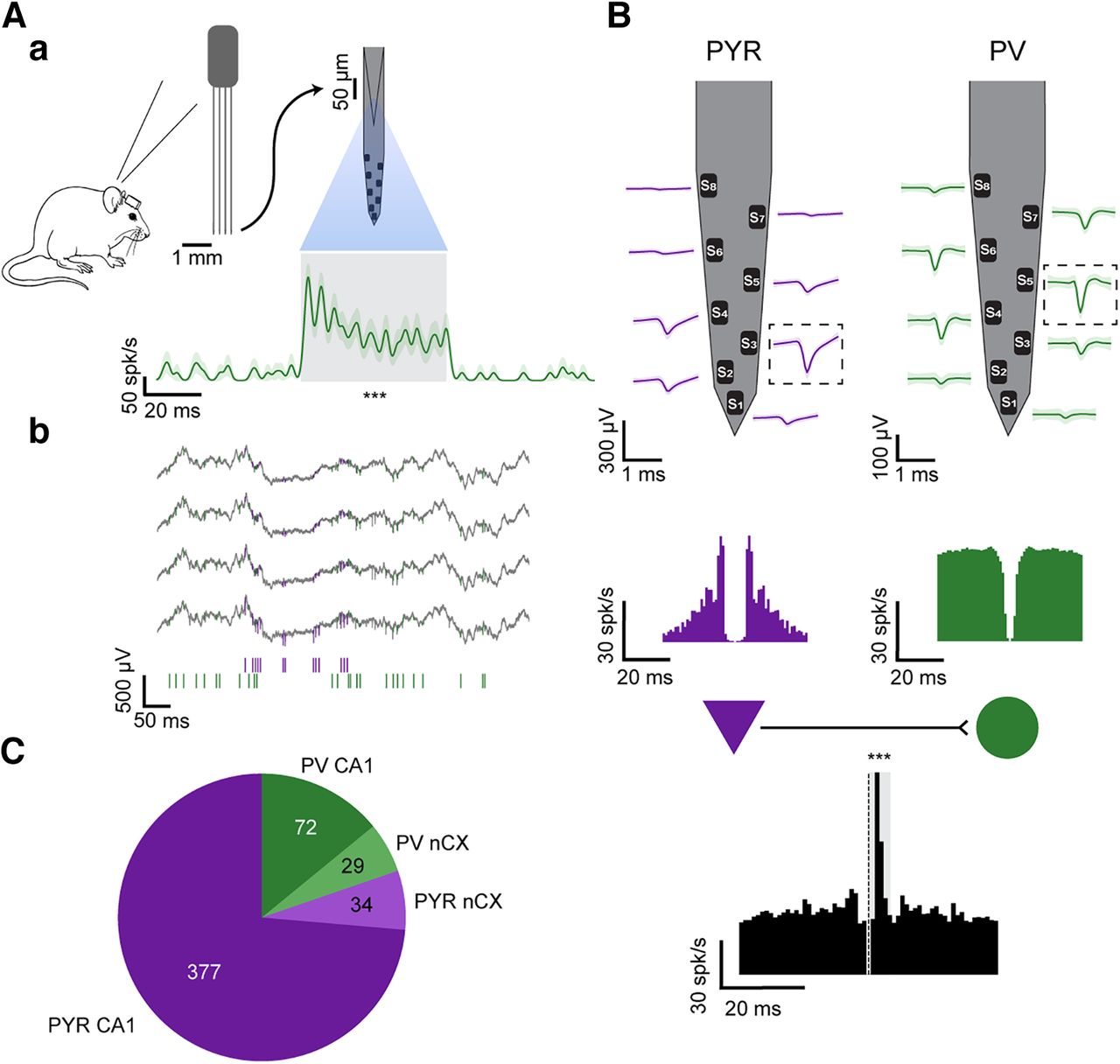
PYR and PV interneurons are tagged in freely moving mice. A, Optical tagging of PV cells. a, Every PV::ChR2 mouse was chronically implanted with a four-fiber/four-shank/32-channel optoelectronic array in the neocortex (nCX). Optical stimuli were applied, in separate sessions, in the nCX and in hippocampal region CA1. Peristimulus time histogram of the PV cell (bottom), triggered by the onset of 50 ms light pulses applied on the optical fiber attached to the recording shank (n = 20; 33 μW). The unit is tagged as PV because of a robust firing rate increase during light (gray) compared with no-light periods. ***p < 0.001, Poisson test. b, Wide-band (1–5000 Hz) recordings from four same-shank channels in CA1. Bottom, Spike trains of a PYR (purple) and the PV cell (green). B, Connectivity-based tagging. Top, Mean (±SD) spike waveforms. For every unit, the channel that exhibits the highest trough-to-peak magnitude is denoted the main channel (boxed). Middle, Auto-correlation histograms (ACHs), showing burst spiking activity of the PYR (purple). Bottom, Cross-correlation histogram (CCH; black) between the spikes of the PYR and the optically tagged PV cell. Gray, Monosynaptic window. The CCH is consistent with monosynaptic excitation of the PV cell by the reference unit, tagging the reference unit as excitatory (PYR). ***p < 0.001, Poisson test. C, Tagged dataset. Of the 512 units in the dataset, 411 (80.3%) are PYR, and 449 (87.7%) are from CA1.
- Figure 2.
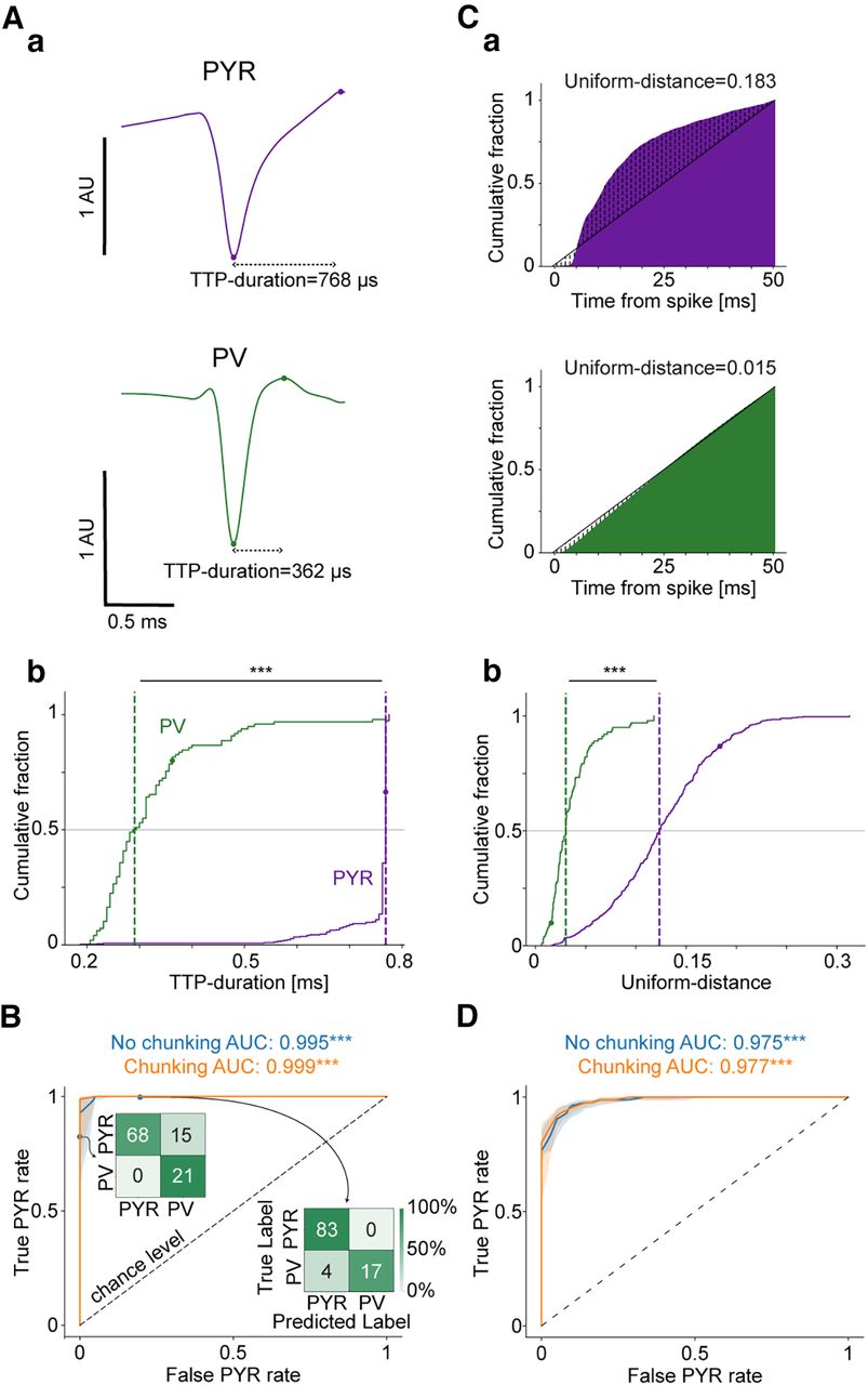
Waveform-based and spike-timing features allow near-perfect classification of PYR and PV cells. A, Features extracted from the mean waveform of the main channel. Voltage values were scaled by the absolute value at the maximal negativity, yielding arbitrary units (AU; the example units are the same as in Fig. 1B). a, Trough-to-peak (TTP) duration feature, defined as the time between the maximal negativity and the ensuing maximal positivity. b, Cumulative distribution function (CDF) of the TTP duration feature for the entire population (PYR, n = 411; PV cells, n = 101; no chunking). Here and in all subsequent CDFs, horizontal lines represent 50%, vertical dashed lines indicate medians, and the *** symbol corresponds to p < 0.001 (U test). The filled circles represent values corresponding to the examples given in a. The difference between PYR and PV cells indicates longer TTP durations for PYR compared with PV cells. B, Waveform-based features allow near-perfect classification. Cross-validated random forest models were trained using the waveform-based features (n = 50 partitions). The chunking method yields improved classification compared with no chunking. The ROC AUCs without chunking (blue) and with 50 spike chunks (orange) are higher than chance level. ***p < 0.001, Wilcoxon test compared with chance level, 0.5. Inset, Confusion matrices (no chunking) based on different decision thresholds (top, 0.1; bottom, 0.9) show variability in prediction, exemplifying the shortcomings of threshold-dependent metrics. C, Features extracted from spike timing. High-frequency features derived from single-sided short-term (0–50 ms) ACHs. a, The Uniform-distance feature is defined as the average absolute difference between the single-sided ACH and a straight line (the example units are the same as in Fig. 1B). b, Cumulative distribution of the Uniform-distance feature for the entire population (no chunking). The larger Uniform-distance values for PYR indicate larger deviations from linear recovery for PYR compared with PV cells. D, Classification based on spike-timing features is not consistently improved by chunking. AUCs were derived from ROC curves based on n = 50 cross-validated random forest models. ROC curves for the test data without chunking (blue) and with 1600 spike chunks (orange) with performance above chance level. All conventions are the same as in B. See also Extended Data Figures 2-1, 2-2.
- Figure 3.
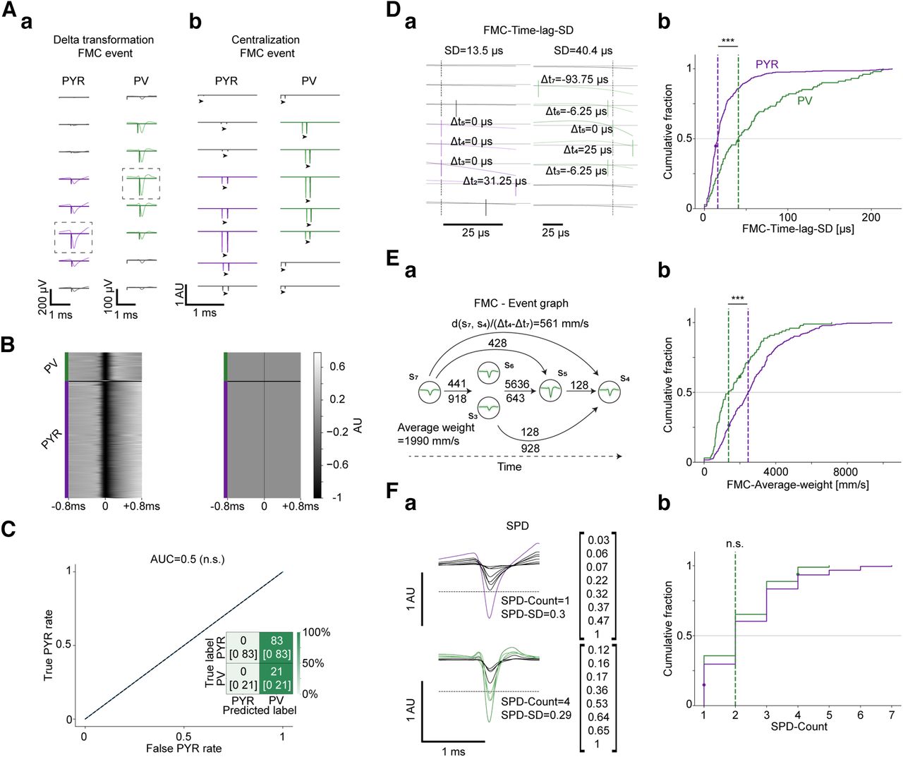
Transforming multichannel spike waveforms to event-based δ-like functions removes all waveform-based information and allows extracting purely spatial features. A, The event-based δ-transformation procedure, illustrated for the FMC event. a, The mean waveforms, with δ-like functions marking the FMCs. The transformation replaces all voltage values with zeros, except for the event points, which are assigned the same value as the trough. In gray are channels for which the magnitude of the TTP is below a predetermined threshold (Materials and Methods). The main channels are boxed. b, Next, waveform-related information that might be recovered by combining multiple δ-transformed events is removed. The δ-like functions are scaled and centralized (arrowheads), placing the event of the main channel at the midpoint (129th sample). B, Left, The scaled waveform of the main channel of all units in the dataset before the transformation, sorted for PYR and PV cells separately by the time of the trough. Right, The same waveforms after event-based δ-transformation. The transformation removes nearly all of the variability between units. C, Cross-validated random forest models (n = 50; no chunking) were trained using waveform-based features extracted from the transformed spikes. The confusion matrix, based on a naive decision threshold of 0.5, yields a constant prediction of one class. n.s.p > 0.05, Wilcoxon test. Numbers in every cell denote the median [IQR]. Performance was quantified by the threshold-independent AUC. The classification yields an AUC of exactly 0.5, corresponding to purely random prediction. D, A time-based feature, FMC-Time-lag-SD, derived from the differences between the times of the FMC event in different channels. The feature quantifies the temporal dispersion of the event, without considering the actual positions of the recording electrodes. a, FMC-Time-lag-SD is defined as the SD of the time differences between the FMC event of the main channel (vertical dotted lines) and the other channels. In gray are ignored channels, for which the magnitude of the TTP was below a predetermined threshold. b, Cumulative distribution of the FMC-Time-lag-SD feature for the entire population (411 PYR, 98 PV cells, no chunking). The smaller FMC-Time-lag-SD values of the PYR indicate higher spatiotemporal synchrony for PYR compared with PV cells. All conventions for the CDFs here and in subsequent panels are the same as in Figure 2A. E, A graph-based feature, FMC-Average-weight, derived from the differences between the FMC event time in different channels and the electrode locations. a, FMC-Average-weight is defined as the average edge weight in the event graph. The event graph is a directed graph with vertices representing the electrodes, and edges representing the transmission speed based on the timing of the events and the location of the electrodes. Only channels that passed the threshold for the magnitude of the TTP were considered. b, Cumulative distribution of the FMC-Average-weight feature (no chunking). The larger values for PYR indicate higher transmission rates for PYR compared with PV cells. F, A value-based feature, SPD-Count, derived from SPD of the maximal negativity on every channel. a, SPD-Count is defined as the number of channels that reached at least 50% of the maximal negativity of the main channel. b, Cumulative distribution of the SPD-Count feature (no chunking). No consistent difference between the PYR and PV cells is observed, suggesting similar spatial distributions of the scaled maximal negativity (p > 0.05, U test). See also Extended Data Figure 3-1.
- Figure 4.
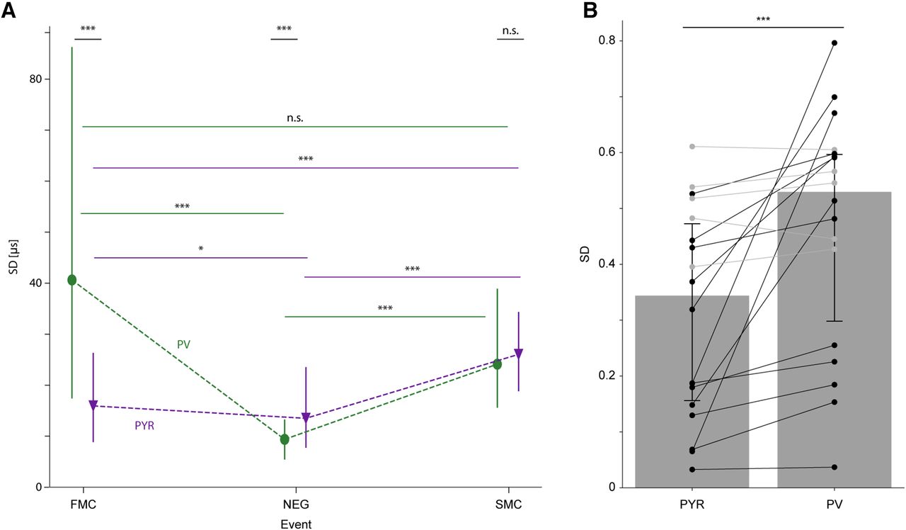
The variance of spatial features over channels and across chunks is different for PYR and for PV cells. A, Variance over channels differs between events and cell types. Compared with PYR, PV cells show lower spatiotemporal spike synchrony (i.e., higher SD) during FMC. The relation reverses during the NEG event. The SD of the SMC event is not consistently different between PYR and PV cells. n.s.p > 0.05, ***p < 0.001, U test. For both PYR and PV cells, synchrony increases from the FMC to the NEG, and then decreases during the SMC. Lined *p < 0.05, ***p < 0.001, Kruskal–Wallis test, corrected for multiple comparisons. B, Variance across chunks differs between cell types. Every dot shows the SD value for a different spatial feature, based on 25 spike chunks. Of 18 features, 13 (72%) differ in the SD values between the cell type groups, with the SD being higher for PV cells (black lines, p < 0.05; gray lines, p > 0.05, U test). Comparing the median SDs of the 18 spatial features between the cell type groups, PV cells exhibit higher SDs compared with PYR. Bars (error bars) represent the median (IQR) of the median feature values for each cell type. ***p < 0.001, two-tailed Wilcoxon test. See also Extended Data Figure 4-1.
- Figure 5.
Features based exclusively on spatial information allow accurate classification of PYR and PV cells. A, Classification based on spatial features is boosted by chunking. AUCs were derived from ROC curves based on n = 50 cross-validated random forest models. The AUC increases monotonically when chunk size is reduced. Every boxplot shows the median (IQR), whiskers extend for 1.5 times the IQR in every direction, a plus indicates an outlier, and notches represent 95% confidence intervals based on bootstrapping with 1000 repetitions. The best performance (highest AUC) and largest improvement compared with no-chunking (∞) is observed for 25 spike chunks. ***p < 0.001, Wilcoxon test. B, Spatial features allow accurate classification. ROC curves for the test data without chunking (blue) and with 25 spike chunks (orange). The AUCs are higher than chance level. All conventions are the same as in Figure 2B. C, Feature importance analysis for spatial models with 25 spike chunks. SHAP values were used to assess the individual contribution of each feature to the prediction. The dotted lines represent chance-level importance values, based on models trained with shuffled PYR-PV labels. The features derived from the FMC event are associated with the highest SHAP values, indicating that synchrony at the initial depolarization phase makes the highest contribution to classification outcome. **p < 0.01, ***p < 0.001, one-tailed permutation test. See also Extended Data Figure 5-1.
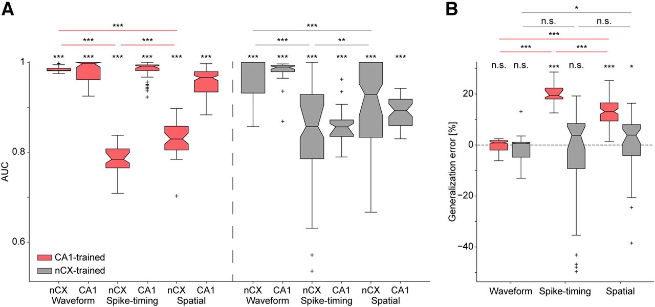
- Figure 6.
Spatial models generalize poorer than waveform models, but better than spike-timing models. A, Cross-validated random forest models (n = 50) were trained for every modality on the CA1 (left, red) or neocortex (nCX; right, gray) data, and tested separately on different data from CA1 and from nCX. Conventions for boxplots here and in B are the same as in Figure 5A. All models exhibit above-chance performance. ***p < 0.001, Wilcoxon test. The performance of models on the non-trained-on region is highest for waveform-based models and lowest for spike-timing models. **p < 0.01; ***p < 0.001, Kruskal–Wallis test corrected for multiple comparisons. B, The decrease in performance on generalization. Generalization error is defined here as the difference between the AUC on the test set of the training region and the AUC on the test set of the non-trained-on region, divided by AUC on the test set of the training region. Spatial models trained on either region and spike-timing models trained on CA1 data, show generalization errors larger than zero. n.s.p > 0.05; **p < 0.01; ***p < 0.001, Wilcoxon test. The dashed horizontal line represents the zero-mark (i.e., same performance on CA1 and nCX). When trained on CA1 data (red), spatial models generalize poorer than waveform models but better than spike-timing models. n.s.p > 0.05; *p < 0.05; ***p < 0.001, Kruskal–Wallis test corrected for multiple comparisons. See also Extended Data Figures 6-1, 6-2.


Tables
Feature Family Description PYR
median [IQR]PV
median [IQR]Effect
size (Aw)aCell type
(p-value)bSHAP
(p-value)cTTP duration Waveform The duration between the trough (maximal negativity) and the peak (maximal positivity) [ms) 0.77 [0.76–0.77] 0.29 [0.25–0.35] 0.98 5.9 × 10−58 0.25 (0.001) TTP magnitude The difference between the trough and the peak (AU)d 1.4 [1.4–1.5] 1.3 [1.2–1.3] 0.97 3.7 × 10−48 0.11 (0.003) FWHM The duration in which the value is at least −0.5 (i.e., half of the trough) (ms) 0.21 [0.2–0.23] 0.16 [0.15–0.18] 0.89 3.7 × 10⁻³⁴ 0.005 (0.59) Rise coefficient A straight line connects the trough and the last sample. The coefficient is the time from the trough to the point where the absolute distance from the line is maximal (ms) 0.29 [0.26–0.32] 0.24 [0.21–0.26] 0.80 2.2 × 10⁻²¹ 0.005 (0.99) Maximum speed First time derivativee The duration after the trough, for which the spike maintains the same change rate (derivative) (ms) 0.19 [0.14–0.26] 0.14 [0.13–0.17] 0.69 3.4 × 10⁻⁹ 0.011 (0.41) Break
measureSecond time derivativee The sum of the values of the second derivative just before the trough (0.3-0.08 ms before the trough) (10–1 *AU) −0.67 [−0.76 to −0.56] −0.58 [−0.7 to −0.49] 0.64 7.9 × 10⁻⁶ 0.003 (0.84) Smile-cry The sum of the values of the second derivative at the end of the spike (0.26-0.76 ms from the trough) (10–2 *AU) −1.2 [−1.4 to −1.1] −0.3 [−0.9 to −0.1] 0.89 5.7 × 10⁻³⁵ 0.013 (0.044) Acceleration The sum of the squared values of the second derivative just after the trough (0.08-0.25 ms after the trough) (10–6 *AU)b 9 [5–14] 91 [49–139] 0.97 6.8 × 10−49 0.12 (0.002) ↵a Aw ranges from 0.5 (no difference) to 1 (nonoverlapping distributions).
↵b Mann–Whitney U test.
↵c Median SHAP values based on 50 spike chunks, indicating feature importance. In parentheses are p-values based on a one-tailed permutation test.
↵d The waveforms are scaled to the −1 to 1 range. Thus, while the original units are μV, here we use arbitrary units (AU).
↵e Derivatives were computed numerically as the difference between every two adjacent samples.
Feature Family Description PYR
median [IQR]PV median
[IQR]Effect
size (Aw)aCell type
p-valuebSHAP
(p-value)cUniform-
distanceHigh frequency
(0–50 ms)dThe mean distance between the CDF of the ACH and the CDF of a uniform distribution 0.12 [0.09–0.16] 0.03 [0.02–0.04] 0.95 1.6 × 10−44 0.14 (0.002) DKL-Short The DKL between the PDF of the ACH and the PDF of a uniform distribution 0.25 [0.17–0.34] 0.058 [0.037–0.079] 0.95 2.2 × 10−44 0.025 (0.36) Rise time The duration in which the values in the CDF of the ACH are above a threshold of 1/e (ms) 11.1 [9.4–13.7] 19.3 [17.8–20.6] 0.88 4.3 × 10⁻³³ 0.031 (0.25) Jump-index Low frequency
(50-1000 ms)dThe mean distance between the CDF of the ACH and the CDF of a uniform distribution 0.067 [0.044–0.088] 0.016 [0.0095–0.024] 0.92 9.3 × 10−39 0.029 (0.31) DKL-Long The DKL between the PDF of the ACH and the PDF of a uniform distribution 0.069 [0.032–0.15] 0.0039 [0.0017–0.012] 0.89 6.1 × 10⁻³⁵ 0.19 (0.001) PSD-center Wide-band
(0–1000 ms)The centroid of the power spectral density (PSD), namely the squared FFT of the ACH (Hz) 37 [33–42] 31 [26–37] 0.65 2.8 × 10⁻⁶ 0.016 (0.56) PSD′-center The centroid of the derivativee of the PSD with respect to frequency (Hz) 23 [19–29] 21 [18–27] 0.57 0.012 0.009 (0.83) Firing rate The average firing rate (spikes/s) 0.69 [0.35–1.47] 8.95 [3.39–16.35] 0.93 1 × 10−40 0.077 (0.038) ↵a Aw ranges from 0.5 (no difference) to 1 (nonoverlapping distributions).
↵b Mann-Whitney U test.
↵c Median SHAP values based on 1600 spike chunks, indicating feature importance. In parentheses are p-values based on a one-tailed permutation test.
↵d Most high-frequency and low-frequency features are based on distributions and therefore hold no units.
↵e Derivatives were computed numerically as the difference between every two adjacent samples.
Feature Family Description Event PYR median [IQR] PV median [IQR] Effect
size (Aw)aCell type
p-valuebSHAP
(p-value)cTime-lag-SS Time basedd The mean SS of the time offsets of the event
(103 * μs2)FMC 0.44 [0.13–1.39] 3.33 [0.49–12.02] 0.74 6.47 × 10⁻¹⁴ 0.094 (0.001) NEG 0.34 [0.1–1.1] 0.16 [0.05–0.35] 0.64 7.04 × 10⁻⁶ 0.008 (0.32) SMC 1.9 [0.77–3.45] 1.69 [0.68–3.48] 0.51 0.34 0.046 (0.015) Time-lag-SD The SD of the time offsets of the event (μs) FMC 15.9 [8.8–26.3] 40.6 [17.4–86.3] 0.72 2.3 × 10⁻¹² 0.093 (0.001) NEG 13.5 [7.7–23.5] 9.4 [5.4–13.3] 0.63 3.44 × 10⁻⁵ 0.009 (0.30) SMC 26 [18.8–34.3] 24.1 [15.6–38.9] 0.50 0.47 0.052 (0.006) Average-weight Graph-based The average edge weight in the graph (mm/s) FMC 2455 [1366–3509] 1206 [684–2577] 0.68 1.65 × 10⁻⁸ 0.038 (0.027) NEG 2724 [1678–4269] 3633 [2173–5387] 0.61 3.13 × 10⁻⁴ 0.007 (0.31) SMC 1844 [1232–2674] 2034 [1099–2947] 0.51 0.34 0.008 (0.31) Longest path The sum of weights in the longest path in the graph (mm/s) FMC 6722 [3581–11,514] 4909 [2417–9945] 0.58 0.0053 0.014 (0.18) NEG 8103 [4200–14,436] 11,517 [4923–16,349] 0.55 0.06 0.006 (0.33) SMC 6050 [3269–11,115] 6888 [3237–11,056] 0.51 0.33 0.013 (0.21) Shortest path The sum of weights in the shortest path in the graph (mm/s) FMC 1049 [657–1619] 494 [267–928] 0.74 1.04 × 10⁻¹³ 0.068 (0.001) NEG 1071 [714–1754] 1607 [916–2572] 0.63 1.4 × 10⁻⁵ 0.006 (0.33) SMC 584 [426–872] 701 [409–1024] 0.55 0.08 0.008 (0.30) SPD- Count Value-basede The number of values that crossed 0.5 2 [1–3] 2 [1–3] 0.55 0.06 0.007 (0.17) SPD-SD The SD of the vector 0.30 [0.28–0.33] 0.29 [0.27–0.31] 0.65 3.02 × 10⁻⁶ 0.008 (0.32) SPD-Area The AUCf 1.95 [1.45–2.54] 2.02 [1.64–2.44] 0.52 0.29 0.016 (0.19) SS, Sum of squares.
↵a Aw ranges from 0.5 (no difference) to 1 (nonoverlapping distributions).
↵b Mann-Whitney U test.
↵c Median Shapley additive explanations (SHAP) values based on 25 spike chunks, indicating feature importance. Parentheses, p-values based on a one-tailed permutation test.
↵d Time offsets are relative to the main channel.
↵e Based on the vector of maximal negativity values for each channel, scaled to the 0–1 range. The features are based on counts and thus hold no units.
↵f The area under the curve of the count of channels versus the threshold value.
Feature Event PYR SD (scaled)
median [QR]aPV SD (scaled)
median [IQR]aAwb p-valuec Time-lag-SS FMC 0.065 [0.019–0.22] 0.67 [0.42–0.93] 0.90 8.9 × 10−37 NEG 0.033 [0.011–0.076] 0.037 [0.011–0.21] 0.56 0.022 SMC 0.15 [0.097–0.23] 0.51 [0.25–0.83] 0.83 1.1 × 10⁻²⁵ Time-lag-SD FMC 0.19 [0.093–0.41] 0.80 [0.61–0.94] 0.90 1.3 × 10⁻³⁵ NEG 0.19 [0.10–0.32] 0.23 [0.12–0.48] 0.56 0.02 SMC 0.32 [0.26–0.42] 0.70 [0.50–0.93] 0.85 1.6 × 10⁻²⁷ Average weight FMC 0.61 [0.36–0.84] 0.61 [0.41–0.76] 0.50 0.46 NEG 0.43 [0.28–0.62] 0.48 [0.36–0.68] 0.57 0.016 SMC 0.54 [0.43–0.65] 0.57 [0.40–0.70] 0.53 0.2 Longest path FMC 0.53 [0.31–0.81] 0.60 [0.43–0.86] 0.57 0.016 NEG 0.44 [0.29–0.68] 0.59 [0.37–0.76] 0.60 0.0015 SMC 0.52 [0.34–0.72] 0.55 [0.36–0.75] 0.52 0.22 Shortest path FMC 0.48 [0.22–0.92] 0.45 [0.33–0.67] 0.50 0.47 NEG 0.37 [0.15–0.71] 0.59 [0.27–0.86] 0.65 7.2 × 10⁻⁵ SMC 0.40 [0.26–0.60] 0.43 [0.28–0.68] 0.54 0.097 SPD-Count 0.069 [0–0.35] 0.15 [0.037–0.40] 0.60 0.0013 SPD-SD 0.18 [0.12–0.24] 0.26 [0.19–0.30] 0.68 6.3 × 10⁻⁹ SPD-Area 0.13 [0.10–0.18] 0.18 [0.15–0.24] 0.73 1.1 × 10⁻¹²
Figure 2-1
Extended data for Figure 2. Waveform-based feature interrelations. A, Rank (Spearman’s) correlations between waveform-based features, grouped by families. Most correlations (26 of 28; 93%) differ from zero. Blank, p > 0.05; *p < 0.05; **p < 0.01; ***p < 0.001; permutation test. B, MI between waveform-based features. All pairs (28 of 28; 100%) exhibit MI values that are higher than chance level. ***p < 0.001, permutation test. Inset, Scatter plot of the MI values between pairs of features and the pairwise absolute rank CCs from A with statistics for rank (Spearman’s) correlation. Download Figure 2-1, TIF file.
Figure 2-2
Extended Data for Figure 2. Spike-timing feature interrelations. A, Rank correlations between the spike-timing features grouped by families. Most correlations (27 of 28; 96%) differ from zero. All conventions here and in B are the same as in Extended Data Figure 2-1. B, MI between spike-timing features. All pairs (28 of 28; 100%) exhibit MI values that are higher than chance level. Inset, Scatter plot of the MI between pairs of features and the CCs from A. Download Figure 2-2, TIF file.
Figure 3-1
Extended Data for Figure 3. Spatial feature interrelations. A, Correlations between the spatial features, grouped by families. Eighty percent of the feature pairs (122 of 153) exhibit correlations that differ from zero. All conventions here and in B are the same as in Extended Data Figure 2-1. B, MI between spatial features. Most pairs (126 of 153; 82%) exhibit MI values that are higher than chance level. Inset, Scatter plot of the MI and the absolute CCs from A. Download Figure 3-1, TIF file.
Figure 4-1
Extended Data for Figure 4. Time-lag-SS and Shortest-path features across events and cell types. A, Time-lag-SS features differ between events and cell types. Compared with PYR cells, PV cells show larger feature values during FMC. The relation reverses during the NEG event. The values during the SMC event are not consistently different between PYR and PV cells. For PV cells, feature values decrease from the FMC to the NEG, and then increase during the SMC. For PYR cells, feature values increase between FMC and SMC, and between NEG and SMC. Here and in B, all conventions are the same as in Figure 4A. B, The graph-based shortest-path feature differs between events and cell types. Compared with PYR cells, PV cells exhibit smaller feature values during FMC. The relation reverses during the NEG event. The values during the SMC event are not consistently different between PYR and PV cells. For PV cells, feature values increase from the FMC to the NEG, and then decrease during the SMC. For PYR cells, feature values decrease between FMC and SMC, and between NEG and SMC. Download Figure 4-1, TIF file.
Figure 5-1
Extended Data for Figure 5. Distribution of the six most important spatial features. A, Cumulative distributions of the FMC-Time-lag-SS feature calculated without chunking. Here and in all subsequent cumulative distribution functions, horizontal lines represent 50%, vertical dashed lines indicate medians. n.s.p > 0.05; ***p < 0.001, U test. B, Cumulative distributions of the FMC-Time-lag-SD feature. C, Cumulative distributions of the FMC-Shortest-path feature. D, Cumulative distributions of the SMC-Time-lag-SD feature. E, Cumulative distributions of the SMC-Time-lag-SS feature. F, Cumulative distributions of the FMC-Average-weight feature. Download Figure 5-1, TIF file.
Figure 6-1
Extended Data for Figure 6. Models of all modalities generalize between brain regions. A, Models based on waveform-based features (50 spike chunks) were trained on CA1 data (top) or on neocortical data (bottom). The AUCs were calculated based on n = 50 models. Performance of waveform-based models is above chance level when tested on either CA1 (left) or neocortical (right) samples. Here and in B and C, ***p < 0.001, Wilcoxon test. B, Models based on spike-timing features (1600 spike chunks) were trained on CA1 data (top) or on neocortical data (bottom). Performance of spike-timing models is above chance level when tested on either CA1 or neocortical samples. C, Models based on spatial features (25 spike chunks) were trained on CA1 data (top) or on neocortical data (bottom). Performance of spatial models is above chance level when tested on either CA1 or neocortical samples. Download Figure 6-1, TIF file.
Figure 6-2
Extended Data for Figure 6. Spatial feature importance indicates consistent characteristics across regions. A, SHAP values for the spatial models with 25 spike chunks trained only on CA1 data. The six most important features are the same as the six most important features in the analyses of models trained on the data from both regions (Fig. 5C). B, SHAP values for the spatial models with 25 spike chunks trained on nCX data. The SMC features are the strongest determinants of the predictions for neocortical-trained models. The six most important features are the same as for the CA1-trained data (A) and as for the models trained on the data from both regions (Fig. 5C). Download Figure 6-2, TIF file.
In this issue


