

Abstract
The habenula is an evolutionarily conserved structure of the vertebrate brain that is essential for behavioral flexibility and mood control. It is spontaneously active and is able to access diverse states when the animal is exposed to sensory stimuli. Here we investigate the dynamics of habenula spontaneous activity, to gain insight into how sensitivity is optimized. Two-photon calcium imaging was performed in resting zebrafish larvae at single-cell resolution. An analysis of avalanches of inferred spikes suggests that the habenula is subcritical. Activity had low covariance and a small mean, arguing against dynamic criticality. A multiple regression estimator of autocorrelation time suggests that the habenula is neither fully asynchronous nor perfectly critical, but is reverberating. This pattern of dynamics may enable integration of information and high flexibility in the tuning of network properties, thus providing a potential mechanism for the optimal responses to a changing environment.
Significance Statement
Spontaneous activity in neurons shapes the response to stimuli. One structure with a high level of spontaneous neuronal activity is the habenula, a regulator of broadly acting neuromodulators involved in mood and learning. How does this activity influence habenula function? We show here that the habenula of a resting animal is near criticality, in a state termed “reverberation”. This pattern of dynamics is consistent with high sensitivity and flexibility, and may enable the habenula to respond optimally to a wide range of stimuli.
Introduction
A defining feature of neural circuits is their flexibility. Although anatomic connectivity does not change rapidly in a mature animal, functional connectivity can change within seconds, enabling animals to quickly alter their behavior to deal with changing circumstances. This is made possible in part by the action of neuromodulators (Getting, 1989; Marder, 2012; Bargmann and Marder, 2013). To ensure that functional connectivity is appropriate for a given condition, the release of neuromodulators is tied to a variety of factors, such as the internal state of the animal, external cues, and perceived reward.
The habenula is an epithalamic structure that receives indirect input from several sensory systems (Stephenson-Jones et al., 2012; Cheng et al., 2017; Zhang et al., 2017), is stimulated by punishment or absence of an expected reward (Matsumoto and Hikosaka, 2007; Hong and Hikosaka, 2008; Amo et al., 2014), and has activity that is dependent on the circadian clock (Zhao and Rusak, 2005; Baño-Otálora and Piggins, 2017; Basnakova et al., 2021) and stress levels (Authement et al., 2018). It sends output to a number of structures, including the raphe (Wang and Aghajanian, 1977) and the rostromedial tegmental nucleus (Jhou et al., 2009), which regulate the release of serotonin and dopamine, respectively. Thus, the habenula is well positioned to coordinate release of broadly acting neuromodulators based on a variety of factors. The importance of the habenula is illustrated by a range of defects seen in animals with a lesioned habenula, including an inability to cope with changing circumstances (Thornton and Bradbury, 1989) or to learn effectively (Agetsuma et al., 2010; Lee et al., 2010). The habenula is thus required for behavioral flexibility (Palumbo et al., 2020; Hones and Mizumori, 2022).
How does the habenula process information to efficiently influence behavior? Calcium imaging in zebrafish indicates that neural activity in the habenula is sensitive to various features of sensory input. Different concentrations of odors (Krishnan et al., 2014), as well as wavelengths (Lin, 2015) or levels of ambient illumination (Zhang et al., 2017) trigger different patterns of activity. This can be represented as trajectories in state space, with reproducible trajectories for each stimulus, indicating that sensory stimuli are represented by population activity. Additionally, habenula neurons constantly fire action potentials, even in the absence of sensory stimulation. This was demonstrated in rats using electrical recordings of brain slices, and has also been found in the zebrafish, using two-photon calcium imaging of tethered animals (Jetti et al., 2014; Fore et al., 2018), or CaMPARI (Calcium Modulated Photoactivatable Ratiometric Integrator)-based labeling of freely swimming fish (Fosque et al., 2015). This activity is driven by input from the forebrain (Bartoszek et al., 2021).
The dynamics of spontaneous activity can influence how information is processed. For example, it has been suggested that highly decorrelated firing, also termed “asynchronous irregular activity,” allows a network to respond rapidly to new input, as the effects of previous inputs are quickly dissipated (Van Vreeswijk and Sompolinsky, 1996). Alternatively, the network may reside close to a point of phase transition, as proposed by criticality theory (Beggs and Timme, 2012). However, whether such a state exists in vivo is controversial (Wilting and Priesemann, 2019b). A third possibility is that the network resides at a near critical yet subcritical point between these two regimes, termed reverberation (Wilting and Priesemann, 2018).
To determine the dynamics of the resting habenula, we assess activity using calcium imaging in the zebrafish. The transparency of this system allows imaging in the intact animal. To mitigate inaccuracies that arise from subsampling (Priesemann et al., 2009; Ribeiro et al., 2014), which can lead to failure to detect criticality, we use the MR estimator that was recently described (Wilting and Priesemann, 2018).
Materials and Methods
Ethical statement
Experiments were conducted using protocols approved by the Institutional Animal Care and Use Committee of Biopolis, Singapore (#171215).
Microscopy and image processing
Calcium imaging was conducted on an upright two-photon microscope system (model A1RMP, Nikon) with a 25× water-immersion objective. Fish expressing nuclear-localized GCaMP6s under the control of the elavl3 promoter [i.e., Tg(elavl3:H2B-GCaMP6s); Dunn et al., 2016; age, 7–11 d] were embedded dorsal up in 2% agarose. At this age, sex cannot be determined (Santos et al., 2017). Time-lapse images were collected with no delay between frames, using a resonant scanner. A single plane was recorded at 113 Hz (n = 2) or ∼15 Hz (n = 16) for 10–15 min. The x–y spatial resolution was 0.50 μm/pixel for 113 Hz data and 0.33 μm/pixel for ∼15 Hz data.
All processing steps for the recordings, including motion correction and detection of regions of interest (ROIs), were done using suite2p (Pachitariu et al., 2017) with the ROIs subsequently manually curated to exclude neurons outside the region of the habenula. From the fluorescence signals obtained via suite2p, the corresponding ΔF/F traces were then computed (Jia et al., 2011), following which discrete spikes were inferred using MLspike with gCaMP6s parameters given in the article (Deneux et al., 2016). Over all of the recordings, the number of neurons range from 152 to 252 with a mean value of 205.6.
Avalanche analysis
Neuronal avalanches were computed by summing the neural spike activities across the population, with individual avalanches being separated by periods of silent time bins (i.e., with zero activity). The total number of spikes across one avalanche constitutes the size, while the duration measures the number of time points the avalanche lasts. The power law distribution was fitted and compared against the exponential distribution using the powerlaw package (Alstott et al., 2014). As the mean size given the duration is not a probability distribution, the function was fitted with a simple linear regression in the log scale.
Shape collapse was performed by adapting the procedure described in the study by Marshall et al. (2016) into Python. We began by excluding avalanches whose durations are less than five timesteps, as well as durations whose total number of avalanche samples are less than three. This was followed by computing the average avalanche profile for all durations, after which the durations were rescaled to one. Next, linear interpolation was performed for each avalanche profile at 1000 points across the rescaled duration. This allows the computation of the variance across avalanche profiles through the interpolated points. The shape collapse error could then be computed, defined as the ratio between the mean variance and the squared span of the avalanche profiles. Here the span refers to the difference between the maximum and minimum values over all the avalanche profiles. Using this shape collapse error, we then searched for the parameter γ that minimizes the shape collapse error in the interval 0 ≤ γ ≤ 5 in increasing precision: first in steps of 0.1, then 0.01, and last 0.001.
Branching parameter estimation
A branching process is defined as a process where the number of active units in the next timestep At+1 (i.e., descendants) is on average a constant multiple of the active units in the current timestep At (i.e., ancestors). We denote this constant m, which is also called the branching parameter. Mathematically we represent it as follows:
Under spatial subsampling, the conventional way of simply regressing the time series at one timestep apart (i.e., At+1 against At) fails to accurately determine m. Here we make use of the multistep regression (MR) estimator of m that has been proven to be consistent even under severe binomial subsampling (Wilting and Priesemann, 2018). To do so, linear regressions were performed for all pairs of At+k against At for all k = 1, …, kmax to obtain slopes rk. It has been shown that while under full sampling we have
The true m can then be readily estimated by curve fitting rk against k using this equation. We note that since 0 ≤ m ≤ 1, this relation is in general an exponential decay function, except when m = 0 or 1. mk can also be rewritten as e– kΔt /τ (Wilting and Priesemann, 2018), where τ = – Δt/log m denotes the autocorrelation time of the process and Δt is the timescale of the data (i.e., the time interval between each measured timestep). τ diverges at criticality (when m = 1), and otherwise still yields information about the timescale at which the influence of a perturbation remains in the system.
Tests on nonstationarity and Poisson activity
As with most statistical estimations for time series, this estimator is valid only when the time series is stationary. We applied a series of tests to identify common sources of nonstationarities (tests 1–3) and to check for the possible presence of Poisson activity (test 4; Wilting and Priesemann, 2018). Our aim was to ensure that the branching process is able to describe the dynamics present in the data. The following was done. (1) We tested the original exponential model
Nonstationarities are uncovered when any of the computed Hoffset, Hτ, or Hlin values is positive. MR estimation is considered valid when Hoffset, Hτ, Hlin, and HMR_invalid values are all negative (regardless of Hpoisson). When both HMR_invalid and Hpoisson values are positive, the procedure is valid with the conclusion that the system exhibits Poisson activity (i.e., m = 0). On the other hand, if HMR_invalid is positive but Hpoisson is negative, then MR estimation is not valid and no further conclusion can be made on the activity.
Spike count covariance
The spike count covariance was computed as described in the study by Dahmen et al. (2019). First, each dataset was divided into N subsets, and the total activity was computed for each neuron in each subset, which we denoted as
We can probe how far the system is to the dynamically balanced critical state through λmax, which measures the largest (and therefore most unstable) eigenvalue of the underlying connectivity matrix of the network. The critical point occurs at λmax = 1. It is given by Dahmen et al. (2019), as follows:
Data availability
Multistep regression was performed using the MR estimator toolbox (Spitzner et al., 2021). The remaining codes used for computation in this study are available at GitHub (https://github.com/suryadi-t/reverberating_habenula). All computations were performed on an HP Z440 Workstation (3.70 GHz CPU) with the 64 bit Windows 10 Education OS.
Results
Analysis of avalanches fails to provide evidence of criticality
We first asked whether there is evidence for criticality in the habenula. One signature of criticality is the presence of neuronal avalanches, which is defined as cascades of neuronal activity between periods of silence, with duration and size distributions exhibiting power laws. Two-photon calcium imaging was used to monitor spontaneous activity in the zebrafish habenula (Fig. 1A), as visible light used in confocal microscopy causes an evoked response (Dreosti et al., 2014). Upon recording a single plane of neurons in the habenula (at ∼15 Hz) and using MLspike to infer spiking activity in the neurons, we found that at least one neuron was active at any given frame for all 16 recordings (Fig. 1C,D). This lack of silent time bins, which implies a lack of avalanches, could be because of the slow rate of recording. We thus made additional recordings at 113 Hz. These yielded periods of inactivity (Fig. 1E,F): two 10 min recordings yielded 360 and 207 distinct avalanches. These observations suggest that avalanches exist in the habenula.

Characterization of neuronal avalanches in the habenula. A, The habenula of Tg(elavl3:H2B-GCaMP6s) fish, imaged at 15 Hz. Scale bar, 25 μm. B, Population statistics (mean and standard deviation, SD) of the neuron average firing rate aggregated over all recordings. The individual firing rate distributions for each recording are given in Extended Data Figure 1-1. C, Activity in a subset of neurons in the habenula imaged at 15 Hz. The black lines indicate frames where there is at least one spike inferred by MLspike. D, Plot showing number of spikes across the population as inferred by MLspike. E, F, Inferred spikes, obtained from imaging a single plane at 113 Hz. E is the entire recording, whereas F is a zoomed in version to a portion. G, H, Distribution of avalanche size (G) and duration (H) in fish imaged at 113 Hz at a single plane. The blue curve is based on data from one fish, while the orange curve is derived from a second fish. The log-log plots are not linear, indicating the absence of a power law. Further avalanche analyses are given in Extended Data Figure 1-2.
Figure 1-1
Average firing rate distributions for each recording computed from the discrete spikes inferred using MLspike. Download Figure 1-1, TIF file.
Figure 1-2
Further avalanche analysis. Top row, Mean avalanche size given duration. Bottom row, Avalanche shape collapse. We see that β and γ are far from satisfying Equation 10, further indicating that the habenula is not critical. Download Figure 1-2, file.
It is predicted from scaling theory (and verified experimentally) that critical avalanching systems manifest power law distributions for both the avalanche size (S) and duration (T; Beggs and Plenz, 2003). In addition, the mean avalanche size given duration
When analyzed with the powerlaw package (Alstott et al., 2014), the size and duration of these avalanches did not fit a power law (Fig. 1G,H; likelihood ratio test did not favor power law over exponential distribution for all cases with p > 0.1). While we observe that Equation 8 appears to hold in this system (Extended Data Fig. 1-2), this relation is known to be valid quite far from criticality (Friedman et al., 2012), and is therefore insufficient on its own to demonstrate criticality. This can be analyzed further by inspecting the avalanche shape (Extended Data Fig. 1-2). A critical system exhibits self-similarity, which manifests not only power law avalanche distributions, but also avalanche shapes that are, on average, identical across scales. Mathematically, the mean number of spiking neurons s(t, T) at the tth time instant in an avalanche of duration T relates to a universal profile F(t/T) as follows:
By rescaling the durations, these avalanches of different durations could then be collapsed into a universal shape by computing s(t, T)T–γ. In a critical avalanching system, the resulting γ relates to β from Equation 8 in a simple way (Friedman et al., 2012):
We observe in our data that while there is an apparent shape collapse, the shape is flat instead of the parabolic shape predicted by mean field theory, which has also been observed experimentally in neural systems (Friedman et al., 2012; Marshall et al., 2016). In addition, Equation 10 fails to hold here. These observations, particularly the absence of power law distributions in both avalanche size and duration, indicate that the system is not critical.
The MR estimator suggests a subcritical, reverberating state
This lack of evidence for a critical state may be because of subsampling, which was imposed by technical limitations. Specifically, volumetric imaging could not be conducted at a high enough rate, because of delays in focusing across the entire depth of the habenula. We thus used the MR estimator to provide a measure of where the dynamics of the habenula resides in the asynchronous versus critical spectrum. Given that nonstationarities in the data may lead to inaccuracies in the estimation process (Wilting and Priesemann, 2018), we first performed several tests to identify common nonstationarities. These results are indicated in Figure 2, where datasets that passed all stationarity tests are indicated as “Clear” while datasets that did not pass are indicated by the first test they failed. Here the points are expected to follow an exponential decay as given in Equation 2 in the Materials and Methods section, which we observe to be the case, with the red curve in each subplot representing the fit by the exponential decay function. We later show in Extended Data Figure 3-1 that this shape is abolished on temporally shuffling the data.

The regression slopes rk at different time lags k. The blue curve represents actual data, whereas the red curve is the fit using the estimated
Figure 2-1
Simulations of stationary branching process that nevertheless test positive for Hpoisson and
We found a number of datasets that were positive for Hpoisson or HMR_invalid. These tests were conducted to identify regimes of Poisson activity for which rk is expected to be a noisy fluctuation of ∼0, in which case the mean of rk would naturally not be significantly larger than zero, thereby being positive for the tests. In the datasets that tested positive for HMR_invalid and Hpoisson; however, we observe the characteristic exponential decay in line with the prediction for a non-Poisson and noncritical branching process (0 < m < 1), which effectively places these datasets outside of what the two tests are addressing. We therefore hypothesized that these datasets result from stationary branching processes, which are positive for either of the two tests because of fluctuations due to small sample size. This is supported by the observation that the estimated
The accepted datasets were analyzed with the MR estimator, with the results also indicated in Figure 2. The dynamics of the habenula was treated as a branching process, such that the activity in the next timestep At+1 is on average a linear function of that in the current timestep with the addition of some external drive with a mean rate h, as given in Equation 1. As the equation indicates, m encodes the amount of temporal correlation present in the system; the spatial correlation is implicit as this framework considers not individual units, but the total activity over the entire system. When measured in the timescale of neuron activity, m = 0 denotes a state with no temporal correlation (i.e., asynchronous-irregular), while m = 1 denotes a critical state where long-term temporal correlation is observed. When m is close to but not exactly 1 in the neuron activity timescale, the system is situated in a reverberating state that shares some of the benefits of the critical state without its drawbacks (Wilting and Priesemann, 2019b). As m is close to 1 in this regime, it is also characterized by long autocorrelation time.
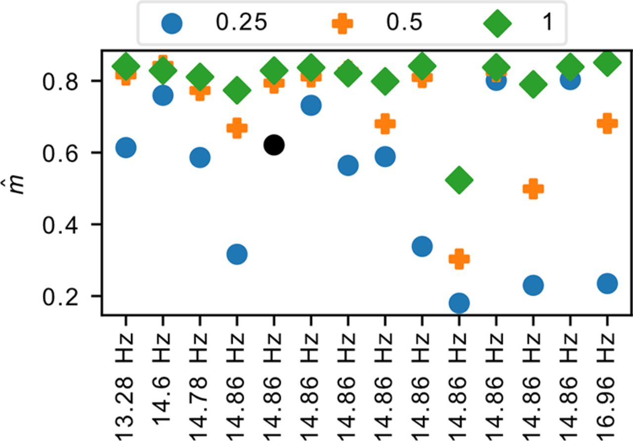
We emphasize that this reverberating state is assessed from m being close to 1 only when measured at the timescale of neural activity. When measured at slower timescales, the inferred value of m changes as it depends on the sampling rate. Specifically, data arising from stationary branching processes should display the branching activity in a systematic way across different timescales within the limits of its autocorrelation time. At different measurement time bins Δt, the inferred branching parameter

Inferred
Figure 3-1
A representative sample of the regression slopes rk at different time lags k for shuffled data. Each row is a specific dataset temporally subsampled to yield multiple effective sampling rates, which progressively becomes noisier as temporal subsampling reduces sample size. In each case, shuffling leads to a noisy horizontal line in the plot clustered at ∼0, indicating Poisson activity (m = 0). Indeed, the majority test positive for Hpoisson, while the remaining few are positive for other nonstationarity tests. Download Figure 3-1, TIF file.
Since the estimator has been shown to be generally consistent over spatial subsampling in the cortex of mammals using electrical recordings (Wilting and Priesemann, 2018, 2019a), we tested whether this also holds here with calcium imaging data. Interestingly, we observe that to be not the case, as seen in Figure 4. To understand why, we simulated stationary branching processes at mtrue = 0.985 and 0.9999, where the two cases reflect reverberating and critical dynamics, respectively. This is followed by temporal subsampling by a factor of 15, as neural activity timescale is approximately ΔT = 4 ms (Wilting and Priesemann, 2019a); this temporal subsampling then brings the measurement timescale to be at Δt = 60 ms, which is close to that of our recordings (approximately Δt = 66–76 ms). In this coarser timescale, the effective values of m become m = 0.7972 and 0.9985, respectively, as per Equation 11. We then performed spatial subsampling in two different ways. In the first case, we spatially subsample by binomial subsampling, where each spike has an equal probability of being “skipped” because of subsampling. We used this as a basis since MR estimator was proven to be consistent under this type of subsampling. In the second case, we follow actual experimental conditions where there is systematic subsampling of specific neurons. We do so by simulating a simple lattice network of neurons, each connected to four other neurons, and subsample by measuring only a random subset of the neurons. To mimic our experimental conditions, we first subsample the network to 250 neurons (approximately the number measured by our recordings) before investigating how further spatial subsampling affects the inferred
Effect of spatial subsampling on
Figure 4-1
Simulation results showing the impact of different types of spatial subsampling. In all cases, we simulated a system of 15,000 neurons before temporally subsampling by a factor of 15 and spatially subsampling to 250 neurons. Each subplot then shows the impact of further subsampling from this initial population of 250 neurons. A–H, Left column (A, C, E, G), Temporal subsampling by skipping bins; right column (B, D, F, H), temporal summation by summing over skipped bins. A–D, Spatial subsampling by binomial subsampling (i.e., skipping individual spikes). E–H, Systematic subsampling by skipping neurons. A, B, E, F, mtrue = 0.9999, m = 0.9985; C, D, G, H, mtrue = 0.985, m = 0.7972. Download Figure 4-1, TIF file.
After verifying this, we reconsidered the process of temporal subsampling compared with our experimental conditions. Temporal subsampling is typically achieved by measuring a subset of the original data. When subsampling by a factor of n, for every n consecutive data points, we measure the nth element and discard the rest. The situation here, however, differs. Because of the slow decay time of gCaMP6s, MLspike would in principle be able to capture the spikes that occur in between time bins. In this case, then, for every n consecutive data points, we measure the sum over all n elements instead, resulting in a form of temporal summation. The right column of Extended Data Figure 4-1 shows the impact of this temporal summation. In most cases, we see that the MR estimator retains its consistency; however, we see in one case that it begins to systematically underestimate m with severe spatial subsampling. This is in fact the case that corresponds most with our setting: m = 0.7972 (mtrue = 0.985) with both temporal summation and systematic subsampling of neurons. The measured
On the other hand, it was also noted that when very few neurons were measured, deviations could also come from heterogeneity within the network (Wilting and Priesemann, 2019a). Our simulations here consist of homogeneous neurons (since we used a lattice topology where every neuron is equivalent), indicating that systematic spatial subsampling can also have an effect on
These findings imply two things. First, our measured
Activity in the habenula has a high autocorrelation time
In the preceding section, we looked at how

Autocorrelation time in the habenula. The autocorrelation time τ (in seconds) for each of the accepted datasets, labeled and sorted by the recording sampling rate. The box plot on the right shows the aggregated statistics of these values.
The habenula is reverberating and not critical
We have so far studied the system through the perspective of avalanche distributions and autocorrelation time in branching processes. We asked whether there is additional evidence for the habenula being in a reverberating rather than a critical state. It has been shown that for a state with critical avalanches (i.e., with branching parameter m = 1), the spike count covariance between neurons in the system should be distributed with a mean value far from zero with a relatively small width (Dahmen et al., 2019). What we observe consistently in our system, however, are distributions that are largely symmetrical, ∼0 (Fig. 6, spike count correlation distribution, which normalized the support of the distribution to [–1, 1]). In our datasets, we found that the width is considerably larger than the mean. This finding remains consistent even with further spatial subsampling of the data (Extended Data Fig. 6-1). This is in fact more consistent with another dynamic regime known as the balanced state (Dahmen et al., 2019), which is characterized by an excess of inhibition.

Spike count correlation distribution. Each panel indicates the distribution of a different dataset. For all the accepted datasets, the mean μ is significantly smaller than the width σ of the distribution. This finding is also consistent with further spatial subsampling of the system (Extended Data Fig. 6-1).
Figure 6-1
Spike count covariance distribution of spatially subsampled data. Each row represents a specific dataset spatially subsampled by a factor given by the column. In all cases, we observe consistency in the relationship between the mean μ and the width σ of the distribution. Download Figure 6-1, TIF file.
We next looked into the dimensionality of the underlying dynamics. The dynamics of a critical avalanching system is characterized by a single dominant eigenvalue, leading to an effective dimensionality of ∼1, which can be probed by performing PCA on the spike count matrix of the system (Dahmen et al., 2019) with the effective dimension computed using the participation ratio (Abbott et al., 2011; Mazzucato et al., 2016). We observed that the habenula datasets display a more gradual decay in the explained variance ratio, which yields a larger effective dimension of ∼19.9–26.9 (Fig. 7). In addition, the activity along the different principal components are observed to have heterogeneous loadings (Extended Data Fig. 7-1), which contrasts the expected homogeneous loadings for a critical avalanching system (Dahmen et al., 2019). These observations, together with the preceding sections, strongly indicate that the habenula is not in a critical avalanching state. On the other hand, while the findings here may suggest that the habenula could reside in the dynamically balanced critical regime (the second type of criticality discussed in the study by Dahmen et al., 2019), our analysis revealed that the relevant measure λmax lies significantly below the value that would be expected of such a regime (Fig. 8), indicating that the habenula is also not in the dynamically balanced critical state.

PCA explained variance ratio for the accepted datasets. All cases display a gradual decline instead of just a single dominant contribution, with the effective dimensions being significantly >1. In addition, activity along the different principal components have heterogeneous loadings (Extended Data Fig. 7-1). These deviate from what is expected from a neural system with critical avalanches.
Figure 7-1
Loadings for the top three principal components. Each row represents a principal component, and each column is for a particular sample dataset, truncated to 50 neurons for clearer visualization. In all cases, the loadings are nonuniform with a mix of positive and negative contributions. Download Figure 7-1, TIF file.
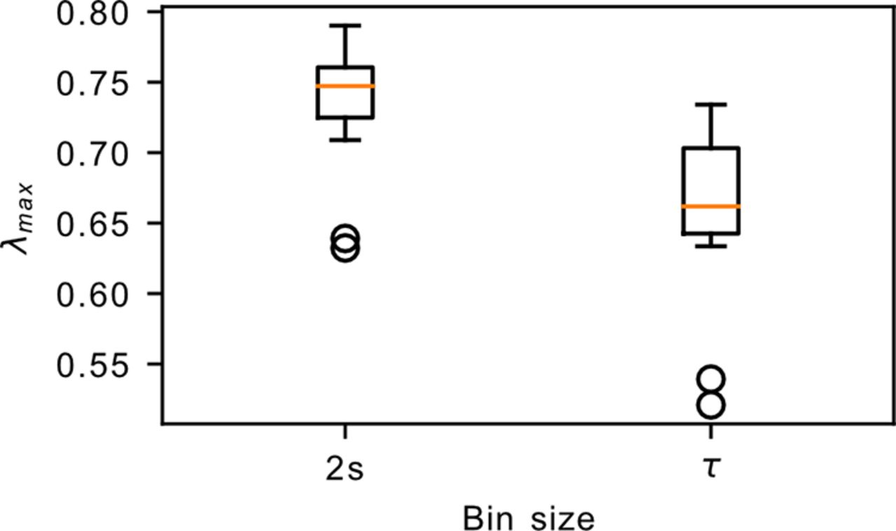
The largest eigenvalue λmax of the connectivity matrix. The computation of λmax requires the binning of the spikes into time bins. This plot shows the results obtained after binning the spikes into 2 s bins, as well as binning into different sizes for each dataset according to its own autocorrelation time τ. In both cases, the λmax values lie well below the critical point at λmax = 1.
Discussion
The dynamics of a system influences how information is processed. Neural networks have in many instances been described as being either critical (Burns and Webb, 1976; Softky and Koch, 1993) or asynchronous (Van Vreeswijk and Sompolinsky, 1996; Brunel, 2000). The whole zebrafish brain has been suggested to operate at criticality, although regional differences were noted (Ponce-Alvarez et al., 2018). Here, we examined dynamics of the habenula in vivo, using calcium imaging at cellular resolution as a proxy for electrical activity. Through the analysis of avalanches, the autocorrelation time, and population statistics, we found no evidence of criticality, although the system is situated near criticality. And although it does display large fluctuation in population activity and long autocorrelation time, which are signatures of being near avalanche criticality, the habenula also bears features of asynchronous activity in the dynamically balanced state. On the one hand, the spike count covariance distribution of the asynchronous state has a small mean and a large width, in contrast to the large mean and small width of the avalanche critical state (Dahmen et al., 2019). Our analysis indicates that the habenula follows the former statistical behavior of asynchronous state. On the other hand, the asynchronous state is also characterized by weak fluctuations and short autocorrelation time on the population level, and this is where the habenula differs. Thus, our results suggest that the habenula is not exclusively critical or asynchronous.
Existing work on the asynchronous state revealed the existence of a second type of criticality representing the edge of chaos (Dahmen et al., 2019). Such a state is characterized, among others, by multidimensional activity that can be probed using PCA. Each mode of activity (projected to a particular principal component) is realized by a mixture of positive and negative neuron contributions of various magnitudes, which observe long autocorrelation times. In contrast, avalanche criticality has dimension typically ∼1, with a single dominant mode given by uniform contribution from all neurons. We observe signs of multidimensional dynamics in the habenula, although we have also shown that the habenula is not situated in this critical point of the second type. Together, our observations indicate that the habenula contains a mixture of characteristics from asynchronous and avalanche dynamics near their respective critical states.
There have been a number of attempts to reconcile the presence of both avalanche and asynchronous dynamics in a network. Simulations show that the incompatible asynchronous and avalanche dynamics can be maintained in the same neuronal network through a balance between excitatory (E) and inhibitory (I) signals at a specified average synaptic strength (Li and Shew, 2020). In other words, a mixture of avalanche and asynchronous neuronal dynamics can result depending on the relative strength of the excitatory and inhibitory synapses (i.e., the I/E weight ratio) and the average synaptic weight. At low I/E weight ratio and weak synaptic strength, the network is near the state of avalanche criticality; while at high I/E weight ratio and strong synaptic strength, it is at the heterogeneous asynchronous state (Ostojic, 2014) near the dynamically balanced critical regime (Dahmen et al., 2019). A system can exhibit characteristics of both avalanching and asynchronous dynamics at a crossover point with a proper balance of E and I (Li and Shew, 2020). This crossover point is not a critical point, which is consistent with what we observe in the habenula.
One interpretation of the dynamics observed is that the habenula is reverberating (Wilting and Priesemann, 2018), as indicated by the inferred m and autocorrelation time. This state is known to combine features from asynchronous and avalanche dynamics (Wilting and Priesemann, 2019a), which has also been observed here in the habenula. The reverberating state, which has been reported previously in mammalian cortical regions, balances the information processing benefits afforded by the critical state, such as sensitivity, but also reduces the drawbacks, such as lower specificity (Wilting and Priesemann, 2019b). A balance of the two may be more optimal for information processing (Wilting et al., 2018). In the reverberating state, small changes in parameter can lead to large changes in the computational properties of the network (Wilting et al., 2018), while the long autocorrelation time may serve as a form of working memory. This is important for adaptation; should there be a sudden change in the environment, the flexibility conferred by the reverberating state will enable optimal change in internal state and thus ensure survival.
Acknowledgments
Acknowledgments: We thank Dr. Mahathi Ramaswamy, Dr. He Chong, and Dr. Chua Khi Pin for helpful discussions and prior explorations leading to this work.
Footnotes
The authors declare no competing financial interests.
This work was funded by the Singapore Ministry of Education through an Academic Research Fund Tier 1 Award (MOE2016-T1-001-152) and a Tier 2 Award (MOE2017-T2-1-058).
This is an open-access article distributed under the terms of the Creative Commons Attribution 4.0 International license, which permits unrestricted use, distribution and reproduction in any medium provided that the original work is properly attributed.
References
In this issue


