Article Figures & Data
Figures
- Figure 1.
Experimental design. A, Data were acquired using a standardized two-photon calcium imaging pipeline based on that described in de Vries et al. (2020) and Groblewski et al. (2020; Materials and Methods). Briefly, a custom headframe was implanted; ISI was performed to delineate retinotopically mapped visual areas; the mouse was habituated to the passive viewing paradigm over the course of approximately two weeks; and two-photon calcium imaging was performed in the left visual cortex while animals viewed stimuli presented to the contralateral eye in several experimental sessions. B, Example of an ISI map. C, Schematic of the two-photon imaging rig (reproduced with permission from Fig. 1D in de Vries et al. 2020). During the imaging sessions, head-fixed mice were free to run on a rotating disk. Locomotion velocity was recorded and pupil diameter was extracted from video of the animal’s right eye. D, Example frame from a two-photon movie. Imaging data were processed as described in de Vries et al. (2020) to obtain ΔF/F0 traces. E, Schematic of the five visual areas targeted in this study. F, Ten randomized blocks of 12 30-s movie stimuli were presented; 4 s of mean-luminance gray was presented between stimuli. The first 60-s period was mean-luminance gray (spontaneous activity); the second 60-s period was a high-contrast sparse noise stimulus (not analyzed in this work). G, Still frames from the eight naturalistic (left) and four artificial (right) movie stimuli (see Materials and Methods, Stimuli). Two of the naturalistic stimuli, “mouse montage 1” and “mousecam,” were phase-scrambled to destroy high-level image features while closely matching low-order statistics (see Materials and Methods, Phase scrambling; Extended Data Fig. 1-1). H, Representative calcium imaging and behavioral data. A heatmap of ΔF/F0 values is shown for 228 neurons simultaneously imaged in L2/3 of AL during presentation of four stimuli, with locomotion velocity and normalized pupil diameter plotted below. Numbers of cells recorded from each layer and area are listed in Extended Data Figure 1-2. Calcium indicator kinetics did not differ across cell populations (Extended Data Fig. 1-3).
- Figure 2.
Spectral differentiation analysis. ND was computed as follows. A, For each cell, the ΔF/F0 trace during stimulus presentation was divided into 1-s windows. B, The power spectrum of each window was estimated. C, The “neurophysiological state” during each 1-s window was defined as a vector in the high-dimensional space of cells and frequencies (i.e., the concatenation of the power spectra in that window for each cell). D, The ND of the response to a given stimulus was calculated as the median of the pairwise Euclidean distances between every state that occurred during the stimulus presentation. An illustration of how the measure behaves is shown in Extended Data Figure 2-1.
- Figure 3.
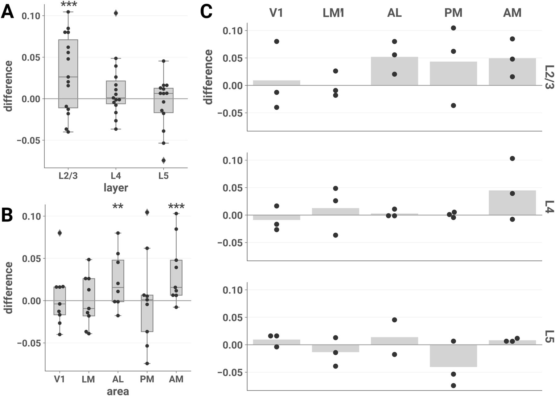
ND elicited by unscrambled versus scrambled stimuli is higher in L2/3 of areas AL and AM. The difference in ND of responses to unscrambled versus scrambled stimuli is plotted for each session by layer (A), area (B), and layer-area pair (C). Each point represents the difference between the mean ND of responses to the two unscrambled and the three scrambled stimuli during a single experimental session. Similar results were found contrasting naturalistic versus artificial stimuli across the entire stimulus set (Extended Data Fig. 3-1). To demonstrate the robustness of this effect, we conducted several further analyses. Sensitivity analyses showed similar findings for various choices of analysis parameters (Extended Data Figs. 3-2, 3-3, 3-4) and when pupil diameter and locomotion were included as covariates in the LME models (Extended Data Figs. 3-5, 3-6, 3-7). We found similar results when we performed the same analysis on discrete calcium events detected from the ΔF/F0 traces with an L0-regularized algorithm (see Materials and Methods, Event detection), indicating that the effect is driven by differences in the large-timescale patterns of responses rather than small-timescale spectral differences within windows (Extended Data Fig. 3-8). Finally, we also found similar results when we removed event-triggered transients from the ΔF/F0 traces, indicating that the effect is not driven solely by initial transients in the calcium response (Extended Data Fig. 3-9). A, B, Asterisks indicate significant post hoc one-sided z-tests in the layer (A) and area (B) interaction LME models (*p < 0.05; ***p < 0.001). Boxes indicate quartiles; whiskers indicate the minimum and maximum of data lying within 1.5 times the interquartile range of the 25% or 75% quartiles; diamonds indicate observations outside this range. C, Mean values are indicated by bars.
- Figure 4.
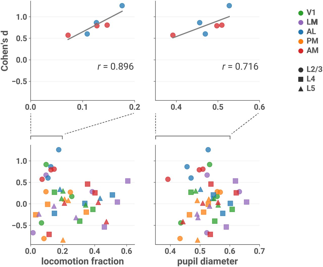
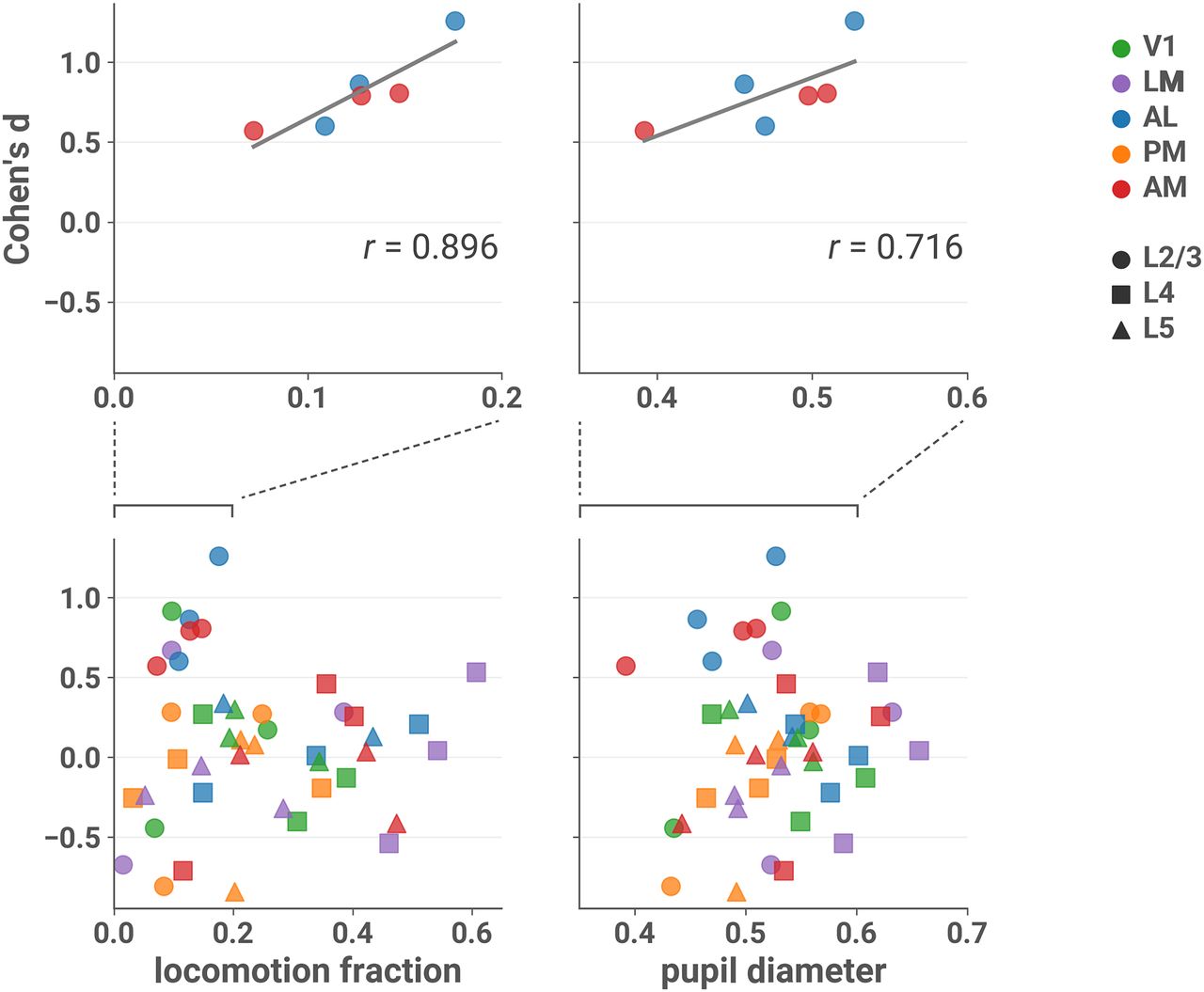
Effect sizes in L2/3 of AL and AM are larger in sessions with more locomotion and larger pupil diameter. Cohen’s d is plotted against the fraction of locomotion activity (left column) and mean normalized pupil diameter (right column) during the session, with linear fit in gray. Top row: only sessions recorded from L2/3 and areas AL or AM. Bottom row: all sessions (note different scales). Top left: Pearson’s r = 0.896 (two-sided t test; t(4) = 4.030, p = 0.0157, 95% CI [0.308, 1.00]l). Top right: r = 0.716 (t(4) = 2.054, p = 0.109, 95% CI [–0.227, 1.00]m). Running velocity >2.5 cm/s was considered locomotion activity (see Materials and Methods, Locomotion). Normalized pupil diameter was obtained by dividing by the maximum diameter that occurred during the session (see Materials and Methods, Pupillometry).
- Figure 5.
Multivariate differentiation analysis. The mean difference in the mean centroid distance of responses to unscrambled versus scrambled stimuli is plotted for each session by layer (A), area (B), and layer-area pair (C). ND elicited by unscrambled versus scrambled stimuli is higher in L2/3 and areas AL and AM, consistent with the spectral differentiation analysis. We found similar results when we analyzed discrete L0 calcium events detected from the ΔF/F0 traces (see Materials and Methods, Event detection; Extended Data Fig. 5-1). A, B, Asterisks indicate significant post hoc one-sided z-tests in the layer (A) and area (B) interaction LME models (**p < 0.01; ***p < 0.001). Boxes indicate quartiles; whiskers indicate the minimum and maximum of data lying within 1.5 times the interquartile range of the 25% or 75% quartiles; diamonds indicate observations outside this range. C, Mean values are indicated by bars.
- Figure 6.
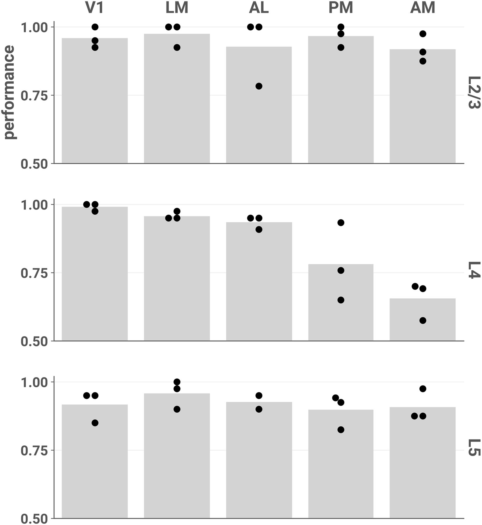
Stimulus category (unscrambled or scrambled) can be accurately decoded from most layers and areas. Each point represents the mean fivefold cross-validated balanced accuracy score of linear discriminant analysis performed on a single session (see Materials and Methods, Decoding analyses). Chance performance is 0.5. We found similar results when decoding stimulus identity across all 12 stimuli (Extended Data Fig. 6-1).
- Figure 7.
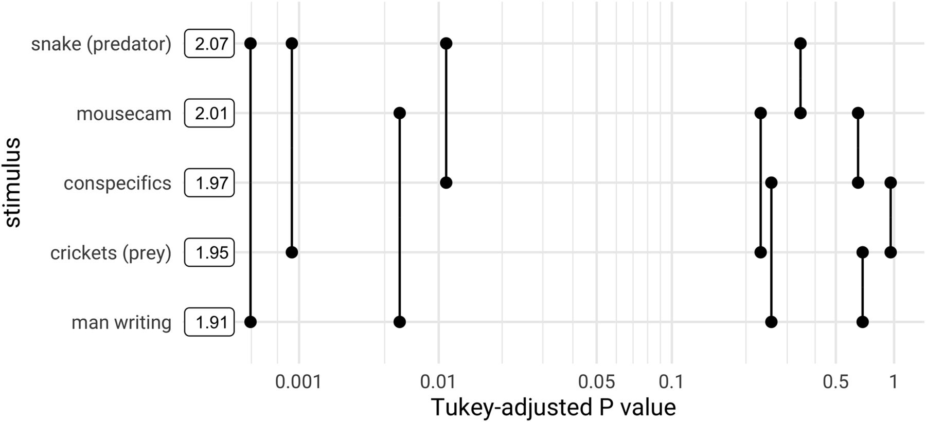
Pairwise differences in ND among unscrambled, continuous stimuli. Post hoc pairwise comparisons using data from all neuronal populations are plotted against their p values (adjusted for multiple comparisons). Boxes show mean ND for each stimulus. ND of the “snake (predator)” stimulus is significantly greater than that of “crickets” and “man writing” at a threshold of α = 0.01, and greater than “conspecifics” at α = 0.05. ND of the “mousecam” stimulus is greater than that of “man writing” at α = 0.01. Mediation analysis showed a mixture of direct and arousal-mediated effects, indicating that changes in arousal cannot fully account for these differences (Extended Data Fig. 7-1). Pairwise differences in ND and decoding performance stratified by layer and area are shown in Extended Data Figure 7-2.
- Figure 8.
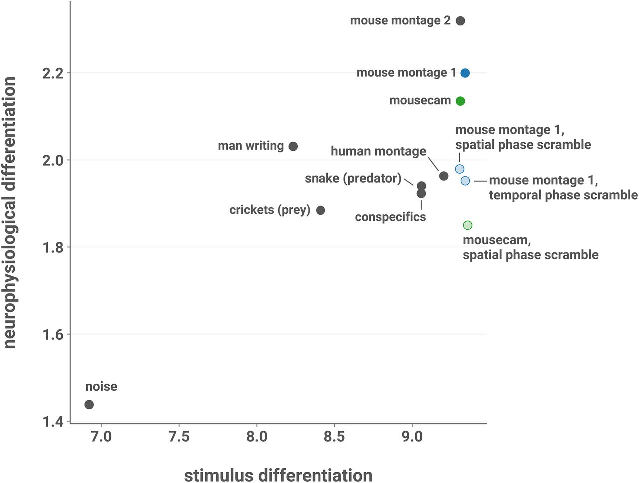
SD does not explain ND. Mean ND elicited by each stimulus in L2/3 of AL and AM, plotted against SD. SD was computed by treating each pixel of the movie as a “cell” and applying the spectral differentiation measure to traces of pixel intensities over time after blurring the movie with a Gaussian filter to account for the coarseness of mouse vision. Across all stimuli, mean ND is positively correlated with SD (Pearson’s r = 0.746; one-sided t test; t(10) = 3.542, p = 0.00267, 95% CI [0.393, 1.00]hh). However, here the noise stimulus is a highly influential observation (Cook’s D = 2.318, an order of magnitude larger than the next most influential observation). With the noise stimulus excluded, the correlation is weaker (r = 0.258; one-sided t test; t(9) = 0.801, p = 0.222, 95% CI [–0.307, 1.00]ii). Moreover, there was no evidence of a relationship with ND when considering only the scrambled stimuli and their unscrambled counterparts (r = –0.378; two-sided t test; t(3) = –0.708, p = 0.523, 95% CI [–0.945, 0.756]jj). ND was also not explained by variation in stimulus luminance, contrast, or spectral energy (Extended Data Fig. 8-1).




Tables
- Table 1
Permutation tests show increased ND for unscrambled versus scrambled stimuli in L2/3 of AL and AM at the level of individual experimental sessions
V1 LM AL PM AM All areas L2/3 1/3 1/3 3/3 0/3 3/3 8/15 L4 0/3 1/3 0/3 0/3 0/3 1/15 L5 0/3 0/3 0/2 0/3 0/3 0/14 All layers 1/9 2/9 3/8 0/9 3/9 Entries contain the fraction of sessions in which the mean ND of responses to unscrambled stimuli was significantly greater than responses to their scrambled counterparts at a threshold of α = 0.05. For each session, a null distribution was obtained by randomly permuting trial labels (unscrambled or scrambled) 20,000 times and computing the difference in mean ND on unscrambled and scrambled trials for each permutation. P values were computed as the fraction of permutations for which the permuted difference was greater than the observed difference.
Data structure Type of test 95% CI a Normal z (one-sided) [0.051, ∞) b Normal z (one-sided) [–0.057, ∞) c Normal z (one-sided) [–0.100, ∞) d Normal z (one-sided) [–0.061, ∞) e Normal z (one-sided) [–0.097, ∞) f Normal z (one-sided) [0.022, ∞) g Normal z (one-sided) [–0.157, ∞) h Normal z (one-sided) [0.128, ∞) i Normal Imai et al. (2010) [0.0784, 0.20] j Normal Imai et al. (2010) [0.0400, 0.15] k Normal Imai et al. (2010) [0.3963, 0.80] l Normal t (two-sided) [0.308, 1.00] m Normal t (two-sided) [–0.227, 1.00] n Normal z (one-sided) [0.0180, ∞) o Normal z (one-sided) [–0.00221, ∞) p Normal z (one-sided) [–0.0189, ∞) q Normal z (one-sided) [–0.0146, ∞) r Normal z (one-sided) [–0.0182, ∞) s Normal z (one-sided) [0.00507, ∞) t Normal z (one-sided) [–0.0167, ∞) u Normal z (one-sided) [0.0163, ∞) v Normal z (one-sided) [0.0158, ∞) w Normal z (one-sided) [–0.00208, ∞) x Normal z (one-sided) [–0.0114, ∞) y Normal z (one-sided) [0.00516, ∞) z Normal z (one-sided) [–0.0198, ∞) aa Normal z (one-sided) [0.00295, ∞) bb Normal z (one-sided) [–0.0170, ∞) cc Normal z (one-sided) [0.0130, ∞) dd Normal t (two-sided) [0.015, 0.180] ee Normal t (two-sided) [0.036, 0.201] ff Normal t (two-sided) [0.076, 0.241] gg Normal t (two-sided) [0.020, 0.185] hh Normal t (one-sided) [0.393, 1.00] ii Normal t (one-sided) [–0.307, 1.00] jj Normal t (two-sided) [–0.945, 0.756]
Extended Data Figure 1-1
Stimuli. Twelve 30-s-long greyscale naturalistic (top) and artificial (bottom) movie stimuli were presented. Left, Montages of six 5-s clips. Right, Continuous 30-s clips. Stimuli used in the main analysis are outlined in blue. Arrows indicate the phase-scrambling procedures. Download Figure 1-1, TIF file.
Extended Data Figure 1-2
Number of cells recorded per layer and area. Download Figure 1-2, TIF file.
Extended Data Figure 1-3
Calcium indicator kinetics did not differ across cell populations. Mean (solid line) ± SD (shaded region) calcium response averaged by (A) layer and area, (B) layer, and (C) area. Calcium responses were obtained for each cell by selecting isolated events (those without any other events occurring in the preceding 50 ms or the following 100 ms) and computing the mean event-locked trace (see Materials and Methods, Event detection). D, Responses were well-fit by an exponential decay function; R2 values of the fit for each cell are plotted by layer and area. E, The fit with the lowest R2 value, 0.61 (cell 5 in session 718673398, L2/3 AM; fit in red, data in black). We tested for a relationship between layer, area, and response half-life by fitting a LME model with layer, area, and their interaction as fixed effects and experimental session as a random effect and comparing this to a model without the interaction term; we found no layer × area interaction (likelihood ratio test; χ2(8) = 1.293, p = 0.996). We tested for main effects of layer and area in two further models and likewise found none (layer: χ2(2) = 1.143, p = 0.565; area: χ2(4) = 0.2288, p = 0.994). Download Figure 1-3, TIF file.
Extended Data Figure 2-1
Differentiation for simulated signals. To illustrate how the ND measure behaves, we generated three artificial signals and computed ND for each. Signals were normalized to have the same energy. A, B, Artificial spike trains were convolved with an idealized GCaMP6f response kernel (difference of exponentials; decay time constant 0.6 s, rise time constant 0.05 s; Chen et al., 2013; Pachitariu et al., 2018) and downsampled to 30 Hz. A, Periodic bursting at 1 Hz. Because the period is the same as the window length used in the spectral estimation step (Fig. 2A), the estimated spectrum of each window is identical, and differentiation is zero. B, An irregular firing pattern has high differentiation. C, Gaussian noise. The theoretical spectrum is identical for each window, but differentiation is nonzero due to the spectral estimation error resulting from the finite window length. Download Figure 2-1, TIF file.
Extended Data Figure 3-1
Naturalistic versus artificial differences in ND across the entire stimulus set. The mean difference in ND of responses to all eight naturalistic versus all four artificial stimuli is plotted for each session by layer (A), area (B), and layer-area pair (C). Results are similar to the unscrambled versus scrambled contrast shown in Figure 3. In this analysis, post hoc tests showed a significant effect also in L5; however, this contrast does not control for low-level stimulus characteristics and is thus harder to interpret. A, We fit an LME model with stimulus category (naturalistic or artificial), layer, and their interaction as fixed effects and found a significant interaction (likelihood ratio test, χ2(2) = 16.343, p = 2.83e–4). Post hoc one-sided z-tests (adjusted for multiple comparisons): L2/3, z = 4.974, p = 9.82e–7, Cohen’s d = 0.153, 95% CI [0.064, ∞); L4, z = –0.450, p = 0.965, Cohen’s d = –0.019, 95% CI [–0.057, ∞); L5, z = 3.745, p = 2.71e–4, Cohen’s d = 0.144, 95% CI [0.037, ∞). B, We fit an LME model with stimulus category (naturalistic or artificial), area, and their interaction as fixed effects and found a significant interaction (likelihood ratio test, χ2(2) = 16.343, p = 0.000283). Post hoc one-sided z-tests (adjusted for multiple comparisons): V1, z = 1.207, p = 0.453, Cohen’s d = 0.066, 95% CI [–0.032, ∞); LM, z = 1.523, p = 0.281, Cohen’s d = 0.074, 95% CI [–0.023, ∞); AL, z = 4.715, p = 6.04e–6, Cohen’s d = 0.222, 95% CI [0.073, ∞); PM, z = –0.907, p > 0.999, Cohen’s d = –0.040, 95% CI [–0.093, ∞); AM, z = 4.249, p = 5.37e–05, Cohen’s d = 0.156, 95% CI [0.056, ∞). A, B, Asterisks indicate significant post hoc tests in the layer (A) and area (B) interaction LME models (***p < 0.001). Boxes indicate quartiles; whiskers indicate the minimum and maximum of data lying within 1.5 times the interquartile range of the 25% or 75% quartiles; diamonds indicate observations outside this range. C, Mean values are indicated by bars. Download Figure 3-1, TIF file.
Extended Data Figure 3-2
Sensitivity analysis of main ND results. We investigated the sensitivity of our results to changes in various parameters of the ND calculation. We systematically varied (1) the distance metric used to compare population state vectors (vertical axis of heatmaps); (2) the length of the window that defines a single state, in which the spectrum is estimated (horizontal axis of heatmaps); (3) the spacing of the frequency bins in the estimated spectrum (linear, A, B; logarithmic, C, D); and (4) the window type and amount of overlap used in estimating the spectra across the stimulus presentation (shown in the following two figures). For each combination of these parameters, we computed ND values and performed the same statistical analysis as described in the main text. Each cell in the heatmaps in A, C shows the p value of the likelihood ratio test for the stimulus category × layer interaction (left) and stimulus category × area interaction (right); cells in B, D show p values for the associated post hoc tests. The results reported in the main text correspond to the second row and third column of the heatmaps in A, B. For nearly all other combinations of parameters, we likewise find that unscrambled stimuli elicit increased ND specifically in L2/3 of AL and AM. Download Figure 3-2, TIF file.
Extended Data Figure 3-3
Sensitivity analysis was performed as described in Extended Data Figure 3-2, except that the time-frequency analysis step of computing ND (Fig. 2A) was performed using a Tukey window with 12.5% overlap. Download Figure 3-3, TIF file.
Extended Data Figure 3-4
Sensitivity analysis was performed as described in Extended Data Figure 3-2, except with a Kaiser window (β = 14) with 50% overlap. Download Figure 3-4, TIF file.
Extended Data Figure 3-5
Sensitivity analysis for LME models including arousal variables (locomotion and pupil diameter) as covariates. Consistent with results from the simpler models, L2/3 of AL and AM emerge as the cell populations in which ND is greater for unscrambled versus scrambled stimuli for nearly all parameter combinations. Download Figure 3-5, TIF file.
Extended Data Figure 3-6
Sensitivity analysis as in Extended Data Figure 3-5, using a Tukey window with 12.5% overlap. Download Figure 3-6, TIF file.
Extended Data Figure 3-7
Sensitivity analysis as in Extended Data Figure 3-5, using a Kaiser window (β = 14) with 50% overlap. Download Figure 3-7, TIF file.
Extended Data Figure 3-8
Spectral differentiation analysis of discrete L0 calcium events. The difference in ND of responses to unscrambled versus scrambled stimuli is plotted for each session by layer (A), area (B), and layer-area pair (C). Results are similar to the main analysis on ΔF/F0 traces shown in Figure 3. This indicates that the differences we observed in ND are driven by differences in the large-timescale patterns of responses rather than small-timescale spectral differences within the windows, consistent with the sparsity of calcium responses in our dataset. A, We fit an LME model with stimulus category (naturalistic or artificial), layer, and their interaction as fixed effects and found a significant interaction (likelihood ratio test, χ2(2) = 11.481, p = 0.00321). Post hoc one-sided z-tests (adjusted for multiple comparisons): L2/3, z = 3.835, p = 0.000188, Cohen’s d = 0.175, 95% CI [0.0478, ∞); L4, z = –0.154, p = 0.916, Cohen’s d = –0.001, 95% CI [–0.0635, ∞); L5, z = –0.507, p = 0.971, Cohen’s d = –0.0318, 95% CI [–0.0761, ∞). B, We fit an LME model with stimulus category (naturalistic or artificial), area, and their interaction as fixed effects and found a significant interaction (likelihood ratio test, χ2(4) = 15.102, p = 0.00445). Post hoc one-sided z-tests (adjusted for multiple comparisons): V1, z = 0.612, p = 0.793, Cohen’s d = 0.076, 95% CI [–0.0483, ∞); LM, z = –0.136, p = 0.982, Cohen’s d = 0.0270, 95% CI [–0.0665, ∞); AL, z = 2.879, p = 0.00995, Cohen’s d = 0.226, 95% CI [0.0329, ∞); PM, z = –1.929, p > 0.999, Cohen’s d = –0.151, 95% CI [–0.161, ∞); AM, z = 2.318, p = 0.05005, Cohen’s d = 0.0984, 95% CI [–0.0179, ∞). A, B, Asterisks indicate significant post hoc one-sided z-tests in the layer (A) and area (B) interaction LME models (**p < 0.01, ***p < 0.001). Boxes indicate quartiles; whiskers indicate the minimum and maximum of data lying within 1.5 times the interquartile range of the 25% or 75% quartiles; diamonds indicate observations outside this range. C, Mean values are indicated by bars. Download Figure 3-8, TIF file.
Extended Data Figure 3-9
Spectral differentiation analysis on ΔF/F0 traces with initial calcium transients removed. Transients were defined as the first 200 ms (6 imaging samples) of the signal after each L0 calcium event. These samples were replaced with linearly interpolated values and ND was calculated for the resulting signal. The difference in ND of responses to unscrambled versus scrambled stimuli is plotted for each session by layer (A), area (B), and layer-area pair (C). Results are similar to the main analysis shown in Figure 3, indicating that our ND results are not driven solely by initial transients in the calcium response. A, We fit an LME model with stimulus category (naturalistic or artificial), layer, and their interaction as fixed effects and found a significant interaction (likelihood ratio test, χ2(2) = 6.024, p = 0.0492). Post hoc one-sided z-tests (adjusted for multiple comparisons): L2/3, z = 2.823, p = 0.00713, Cohen’s d = 0.175, 95% CI [0.0165, ∞); L4, z = 0.850, p = 0.483, Cohen’s d = 0.0568, 95% CI [–0.0299, ∞); L5, z = –0.674, p = 0.984, Cohen’s d = –0.0357, 95% CI [–0.0680, ∞). B, We fit an LME model with stimulus category (naturalistic or artificial), area, and their interaction as fixed effects and found a significant interaction (likelihood ratio test, χ2(4) = 12.886, p = 0.0119). Post hoc one-sided z-tests (adjusted for multiple comparisons): V1, z = 1.032, p = 0.559, Cohen’s d = 0.0946, 95% CI [–0.0390, ∞); LM, z = –0.495, p = 0.997, Cohen’s d = –0.0354, 95% CI [–0.092, ∞); AL, z = 2.911, p = 0.00899, Cohen’s d = 0.257, 95% CI [0.0190, ∞); PM, z = –1.429, p > 0.999, Cohen’s d = –0.0966, 95% CI [–0.114, ∞); AM, z = 2.055, p = 0.0958, Cohen’s d = 0.125, 95% CI [–0.00800, ∞). A, B, Asterisks indicate significant post hoc one-sided z-tests in the layer (A) and area (B) interaction LME models (**p < 0.01). Boxes indicate quartiles; whiskers indicate the minimum and maximum of data lying within 1.5 times the interquartile range of the 25% or 75% quartiles; diamonds indicate observations outside this range. C, Mean values are indicated by bars. Download Figure 3-9, TIF file.
Extended Data 1
Analysis code. All analyses and figures can be reproduced by following the instructions in README.md. Download Extended Data 1, ZIP file.
Extended Data Figure 5-1
Multivariate differentiation analysis of detected calcium events. The mean difference in the mean centroid distance of detected-event responses to unscrambled versus scrambled stimuli is plotted for each session by layer (A), area (B), and layer-area pair (C). Multivariate differentiation elicited by unscrambled versus scrambled stimuli is higher in L2/3 of AL and AM, as well as the additional finding of higher differentiation in L2/3 of V1. A, B, Asterisks indicate significant post hoc one-sided z-tests in the layer (A) and area (B) interaction LME models (*p < 0.05, **p < 0.01, ***p < 0.001). Boxes indicate quartiles; whiskers indicate the minimum and maximum of data lying within 1.5 times the interquartile range of the 25% or 75% quartiles; diamonds indicate observations outside this range. C, Mean values are indicated by bars. Download Figure 5-1, TIF file.
Extended Data Figure 6-1
Stimulus identity can be accurately decoded from most layers and areas using responses to all 12 stimuli. Each point represents the mean fivefold cross-validated balanced accuracy score of linear discriminant analysis performed on a single session (see Materials and Methods, Decoding analyses). Chance performance is 1/12, indicated by the dotted line. Download Figure 6-1, TIF file.
Extended Data Figure 7-1
Mediation analysis of the effect of stimulus. To disentangle the effects of stimulus and arousal on ND, we performed a causal mediation analysis (see Materials and Methods, Mediation analyses). For each of the four stimulus pairs identified as having significantly different levels of ND in our post hoc analysis, we asked whether each of the arousal variables (locomotion or pupil diameter) was a mediator of the effect of stimulus on differentiation, in each case including the other arousal variable as a covariate. The analysis revealed a mixture of direct and mediated effects. Notably, for the largest contrast (predator vs man writing), for both locomotion and pupil diameter we found evidence only for a direct effect. Overall, we conclude that arousal alone cannot account for differences in ND among continuous, naturalistic stimuli. Download Figure 7-1, TIF file.
Extended Data Figure 7-2
Within-category differences in ND versus within-category differences in decoding performance, by layer and area. Top, Cohen’s d for pairwise mean differences in ND among naturalistic stimuli without jump cuts. Bottom, Cohen’s d for pairwise mean differences in stimulus identity decoding performance. For each session, we trained a linear discriminant analysis classifier using only responses to these five stimuli; classification performance was evaluated as the mean fivefold cross-validated F1 score for each stimulus (see Materials and Methods, Decoding analyses). Download Figure 7-2, TIF file.
Extended Data Figure 8-1
ND versus low-level stimulus characteristics. ND is plotted against the mean luminance, contrast, and spectral energy of the stimuli. Mean luminance was computed as the average pixel intensity. Contrast was calculated as the SD of pixel intensities. Spectral energy of the blurred stimuli was computed as the sum of the energy spectral density of each pixel’s intensity timeseries after removing the DC component. Download Figure 8-1, TIF file.
In this issue