


Abstract
Canonical language models describe eloquent function as the product of a series of cognitive processes, typically characterized by the independent activation profiles of focal brain regions. In contrast, more recent work has suggested that the interactions between these regions, the cortical networks of language, are critical for understanding speech production. We investigated the cortical basis of picture naming (PN) with human intracranial electrocorticography (ECoG) recordings and direct cortical stimulation (DCS), adjudicating between two competing hypotheses: are task-specific cognitive functions discretely computed within well-localized brain regions or rather by distributed networks? The time resolution of ECoG allows direct comparison of intraregional activation measures [high gamma (hγ) power] with graph theoretic measures of interregional dynamics. We developed an analysis framework, network dynamics using directed information (NetDI), using information and graph theoretic tools to reveal spatiotemporal dynamics at multiple scales: coarse, intermediate, and fine. Our analysis found novel relationships between the power profiles and network measures during the task. Furthermore, validation using DCS indicates that such network parameters combined with hγ power are more predictive than hγ power alone, for identifying critical language regions in the brain. NetDI reveals a high-dimensional space of network dynamics supporting cortical language function, and to account for disruptions to language function observed after neurosurgical resection, traumatic injury, and degenerative disease.
Significance Statement
This work quantifies the network phenomena of distributed cortical substrates supporting language. First, estimated causality among brain regions was assessed with directed information (DI). Second, a graph theoretic framework extracted task related dynamics from the causal estimates. Finally, we validated these functionally defined networks against the gold standard for causal inference, behavioral disruption with direct cortical stimulation (DCS). We demonstrate that the network measures combined with power have greater predictive capability for identifying critical language regions than discrete, regional power analyses alone.
Introduction
Historically, language has been studied in a localized manner, to attribute specific roles to individual neural substrates. This perspective is evidenced by activity in distinct brain regions measured by the blood-oxygen level-dependent responses of functional MRI (fMRI; Price, 2010) or by high-γ (hγ) power (>60 Hz) in electrocorticography (ECoG) recordings (Crone et al., 2001; Edwards et al., 2005; Towle et al., 2008; Cogan et al., 2014; Conner et al., 2014; Flinker et al., 2015; Riès et al., 2017). Furthermore, lesion studies have demonstrated that different brain lesions separably impair discrete aspects of the language system (Geschwind, 1974; Hickok and Poeppel, 2007). More recently, it is becoming obvious that linguistic processes are better characterized as network phenomena (Fedorenko and Thompson-Schill, 2014; Braun et al., 2015; Medaglia et al., 2015; Bassett et al., 2015; Blank et al., 2016; Domenico, 2017; Herbet and Duffau, 2020), as it has been theorized that network properties better explain the complex and transient dynamics during linguistic cognition (Chai et al., 2016; Herbet and Duffau, 2020; Salehi et al., 2020). We quantified network dynamics during a word generation task to evaluate the hypothesis that linguistic operations engaged during picture naming (PN) are better explained by including the network properties and local activity of specific cortical loci than the activity at each locus itself. Further, we probe whether the critical nature of these sites, evidenced by disruption by direct stimulation is related to their centrality measures within the language network.
Intracranial electrodes in humans provide a unique opportunity to resolve this central debate by enabling direct recordings of neural processes with sufficient temporal resolution and spatial specificity to resolve transient network dynamics. Furthermore, these electrodes can be used to induce targeted transient dysfunction via electrical stimulation, providing causal functional inference. We used both modalities to directly compare regional activation measures (hγ power) with network measures.
ECoG during PN (Fig. 1A) was recorded from subdural grid electrodes implanted in the left language dominant hemisphere of seven patients. We developed a holistic framework, network dynamics using directed information (NetDI), which extracts time-varying network dynamics using information and graph theoretic tools.

A, Multiple (>200) trials of the PN task were performed. For each trial, an image from the Boston naming test (Kaplan et al., 1983) was shown; patient articulated when the image was identified. B, The z scores of mean hγ power responses across trials are shown for a patient in three time windows. B1, In the window 200–456 ms relative to stimulus onset, increased power in visual cortex and decreased power in frontal regions compared with the baseline are observed. B2, The prearticulation window has multiple electrodes with an increase in hγ power in frontal, motor, and temporal regions. B3, The postarticulation window has increase in power in the auditory cortex, aligning with the task wherein the patient hears themselves speak.
DI (Massey, 1990; Kramer, 1998) was used to measure directional information flow between time-series across brain regions. DI measures are valuable in neuroscience (Quinn et al., 2012; Malladi et al., 2016; Murin et al., 2016) given its broad applicability to a wide range of electrophysiological recordings, without model assumptions. Traditional causality metrics like Granger causality (GC; Seth et al., 2015) rely on data belonging to linear auto-regressive models, which ignores nonlinear relationships among brain signals (Kowalik et al., 1996; Stokes and Purdon, 2017). Furthermore, DI is equivalent to GC (Amblard and Michel, 2011, 2012) when the data are truly linear and Gaussian, and it is closely related to Transfer Entropy (Schreiber, 2000; Liu, 2012; Liu and Aviyente, 2012), under the Markov condition. The causality yielded by DI (in bits) is causal in the Wiener–Granger sense (Bressler and Seth, 2011); crucially, no assumptions are imposed on the underlying probability distribution of the data.
This work proceeds in three stages. First, we measured causality between brain regions and extracted task related dynamics from the calculated causality values, to resolve network measures at coarse, intermediate, and fine scales. Second, we evaluated the relationship between network measures and the local power responses. We analyzed the relationships between node centrality, given by “coreness of nodes,” which prior work has identified as a good measure of a node’s influence in the network (Kitsak et al., 2010; Pei et al., 2014; Shin et al., 2016) and hγ power. We also looked at relationships between fine scale measures, in-degrees, out-degrees, and power. These node metrics are the components behind the node centrality measure and throw light on how they influence the node centrality. Third, we evaluated the relationship between whether or not stimulation at a given cortical site disrupted language and its corresponding network measures as estimated by NetDI. Various feature spaces were compared, power feature, network features and combined power and network feature spaces, to examine which feature space has the best discriminability between language positive and language negative areas, based on ground truth data given by clinical functional mapping by direct cortical stimulation (DCS).
Materials and Methods
Picture naming task
Patients performed a PN task, where they were shown images from the Boston naming test (Kaplan et al., 1983). Each trial consisted of an image being displayed on a screen for 2 s, followed by a fixation cross for at three more seconds. Multiple (>200) trials of the PN task were performed for each patient. For each trial, an image from the Boston naming test was shown; patient articulated when the image was identified (details in Table 1). Figure 1A illustrates the experimental methodology.
Data and preprocessing
Intracranial electroencephalography (iEEG) data were obtained from subdural grid electrodes implanted in left hemisphere in patients before resective surgery for intractable epilepsy. Electrodes that had close proximity to the sites of seizure onset, interictal spikes or had >10-dB noise in the 60-Hz band, were considered to be bad channels, and were excluded from the analysis. Also, data from bad trials across all channels were excluded, if the trials included epileptiform activity, or had technical errors. The exclusion of bad electrodes and bad trials were done similar to Conner et al. (2014) and Kadipasaoglu et al. (2014, 2015). Seven patients were analyzed and details of the number of electrodes and the number of trials used for analysis are shown in Table 1, along with patient demographics. iEEG data were preprocessed by first performing a common average reference, where the electrodes within each subject were re-referenced by subtracting the common average of all electrodes (Kadipasaoglu et al., 2017); 60-Hz and higher harmonics were removed using bandstop IIR butterworth filters of order 6. Zero phase filtering was also performed, to ensure that the features in the filtered waveforms were preserved exactly at the same time locations as the unfiltered signals.
Patient information
Analysis time windows
“Stimulus onset” refers to the time at which the picture came on screen, and “articulation time” corresponds to the speech onset time for the verbal response. Data analysis was done in 256-ms windows, and the window before stimulus onset was chosen as the baseline. Windows were called stimulus aligned (SA) or articulation aligned (AA) based on whether the trial data in the window was aligned to the stimulus onset or articulation time, respectively. Windows are denoted as SA/AA: <start time > to <end time > in this article (Fig. 2). For example, AA: −256 to 0 ms represents a window that starts 256 ms before articulation. The 0-ms time has a dual meaning based on the context. It is used to represent stimulus onset in SA windows and articulation time in AA windows. All analyses were done in W = 52 windows, consisting of 11 SA (start times 0–320 ms, sliding by 32 ms) and 41 AA (start times −480 to 768 ms, sliding by 32 ms) windows.

SA windows are aligned to stimulus onset, AA to onset of articulation. The last SA window did not overlap with the first AA window, to ensure temporal continuity. 11 SA (start times 0–320 ms, sliding by 32 ms) and 41 AA (start times −480–768 ms, sliding by 32 ms) windows were used in analysis.
Power analysis
After data pre-processing, the time series from all electrodes were filtered into the hγ band (60–150 Hz) using a zero phase, order 6, IIR butterworth filter, to obtain a hγ signal. In a given SA or AA window, let us denote the raw time-series as  . The hγ signal represented as
  , was obtained after filtering the raw time-series, where N is the length of the hγ time-series in that window (N = 256, since sampling frequency was 1 kHz). For each electrode’s recordings, power was calculated in moving SA time windows over the trial duration, to form a hγ power time series for each trial. The instantaneous power series of hγ power in window w, in a given trial is given by
  . The trial-averaged instantaneous power in window w is
  , where
  and
and  is the mean across the trials. The trial-averaged power series
  in window w were converted into z scores
  , using the mean and SD of the power in the baseline window wb. This resulted in normalized z score power series for SA data. Similarly, z score of power was calculated for AA data. To have responses indexed to both stimulus-driven and articulation-related processes, we used a subset of both SA and AA windows, based on whether we were analyzing data right after the stimulus onset, or around articulation, respectively. Remark: Figure 1 shows power normalized to the trial window (not baseline) solely for visualization purposes, to clearly discern the temporal location of the normalized power responses. For all data analysis involving power, the power was normalized using the baseline window, as described in Equation 1.
 (1)where this
  is the time-average of the power series
  in the window,
  is the mean power in the baseline window wb, and
  is the SD of the baseline power.
Directed Information
DI was estimated in a model free manner using the computationally efficient Kraskov, Stögbauer, and Grassberger (KSG) estimator (Kraskov et al., 2004; Gao et al., 2018), which is based on a k-nearest neighbors (kNN) approach to measuring mutual information (MI). DI was estimated between every pair of channels in each SA and AA time window in a data-driven manner. Every trial was considered to be an independent sample path of an unknown underlying random process, and pairwise DI was estimated using all the trials in a given window. Given two raw time series from a pair of electrodes  and
and  , where
  , DI from
  to
to  is denoted as
  , and is defined as the following:
 (2)where the right hand side of Equation 2 is the conditional MI between time series
  and single sample point Yi, conditioned on the past i – 1 samples
  . DI can also be expressed as sums of conditional differential entropies given by h’s in Equation 2. By definition, differential entropy h(Z) of a continuous random variable Z with a probability density function f(z) is the following:
 (3)
(3)
Also, a conditional differential entropy term can be expressed as a difference of two differential entropies:
 (4)
(4)
From Equations 2, 4, DI can be expanded as the following:
 (5)
(5)
Each entropy term in Equation 5 was estimated using the KSG estimator (Kraskov et al., 2004), which uses a kNN approach, similar to the methodology described in Murin (2017). The implementation of DI was written in MATLAB using the kNN tools from Trentool (Lindner, 2011; Lindner et al., 2011). ECoG data were assumed to be Markovian of order m, i.e., samples only depend on the past m samples. Based on a non-parametric method of estimating memory order for ECoG (Murin et al., 2019), and from other similar work (Malladi et al., 2016; Murin et al., 2016), a memory order of 150 ms was used, achieved by using downsamples of the data for estimation. The final equation used for estimation of DI rate  is given by:

 (6)where m is the number of past samples,
  and
and  are the downsampled versions of X and Y, respectively,
  ’ s are the estimated differential entropies, and
  is the length of the downsampled signal.
Bootstrapping and bias-correction of DI estimate
The bias of the empirical estimation of DI is defined as the difference between the true value of DI and the estimated value of DI. All estimators incur bias because of the amount of data samples being finite. The KSG estimator is known to have a negative bias for small sample sizes (Kraskov et al., 2004). To allow for comparisons of DI values, bias-correction was performed for every DI estimate, analogous to debiasing in GC literature (Barrett et al., 2012; Barnett and Seth, 2014). Bias-correction was performed by generating multiple samples of “zero DI” under the null hypothesis by multiple time shuffles of each trial, of one of the channels X, similar to Diks and DeGoede (2001) and Malladi et al. (2016). This ensured that all temporal dependencies were removed between the two channels, and the estimated null DI was denoted as  . The average null DI estimate was subtracted from the original estimated DI, to obtain the bias-corrected estimate of the information flow from X to Y, denoted as the following:
 (7)where
E is the expectation operator. Henceforth, all pairwise DI values under discussion refer to bias corrected values, denoted by
(7)where
E is the expectation operator. Henceforth, all pairwise DI values under discussion refer to bias corrected values, denoted by  to represent information flow from channel X to channel Y, in time window w.
Multiscale graph theoretic framework
A graph theoretic framework (Bullmore and Sporns, 2009, 2012; Sporns, 2010) was used to evaluate connectivity between brain regions. We construct a graph Gw = (V,E) in time window w, where V is the set of M nodes in the graph that represent brain electrodes, E is the set of edges that denote connections between the nodes. The  element of the adjacency matrix
  is given by the directed edge metric from node u to node v, defined as the change in DI from the baseline window. Thus,
  , where b represents the baseline window and N the length of the time window. The edge metric captures the “change in DI from baseline” and represents the changes occurring because of the task dynamics. For each of the seven patients, a total of W(=52) brain graphs were obtained from 52 time windows (11 SA and 41 AA windows). To control for spurious edges, the adjacency matrices were thresholded using a combination of density thresholding and global thresholding techniques (van Wijk et al., 2010). Density thresholding for an adjacency matrix is a technique where the threshold is chosen such that the resulting network has a certain density of edges. Global thresholding for a group of graphs uses a single threshold value (T), and retains all the edges greater than the common threshold. In this work, density thresholding is done in one time window, to determine what T should be, and is then applied globally for all the time windows. Density thresholding was done on a graph corresponding to the window before articulation (AA: –256 to 0 ms), by retaining only the top 5% of the positive increases in DI values, among all pairs of nodes. The cutoff value determined the patient-specific threshold (T), which was then globally applied to all the remaining W – 1 windows. The window AA: –256 to 0 ms was chosen because of its high density of connections, to be very stringent and have a high value of threshold T. The results were found to be largely independent of the window chosen for density thresholding, as using a different window only changed the value of T slightly, which affected a few individual connections, but it was not sufficient to change the subsequent graph theoretical metrics. After thresholding, the elements of the adjacency matrix Aw(u,v) for window w are given by
 (8)and the edges now represent “increase in DI from baseline.” This thresholding technique retains values of DI that are much greater than baseline, and discards “decreases in DI from baseline.” This makes the adjacency matrices positive, allowing for the use and interpretation of most graph processing techniques. The final results are carefully interpreted within the framework of networks built out of increased information flow among brain regions. For each patient, the resulting time varying graphs were analyzed using a multiscale analysis procedure (Fig. 3) using metrics that shed light on the underlying process at various scales, coarse, intermediate, and fine (Fig. 4).

A, Coreness of a node is a measure of the node’s centrality in the network. While typically, a higher coreness value corresponds to a higher node degree, it is not always the case. For example, both nodes P and Q have a degree of 6, yet node P has a coreness value of 1, while node Q has a coreness value of 3. B, Louvain communities. C, Fine scale network measures given by in-degrees and out-degrees.
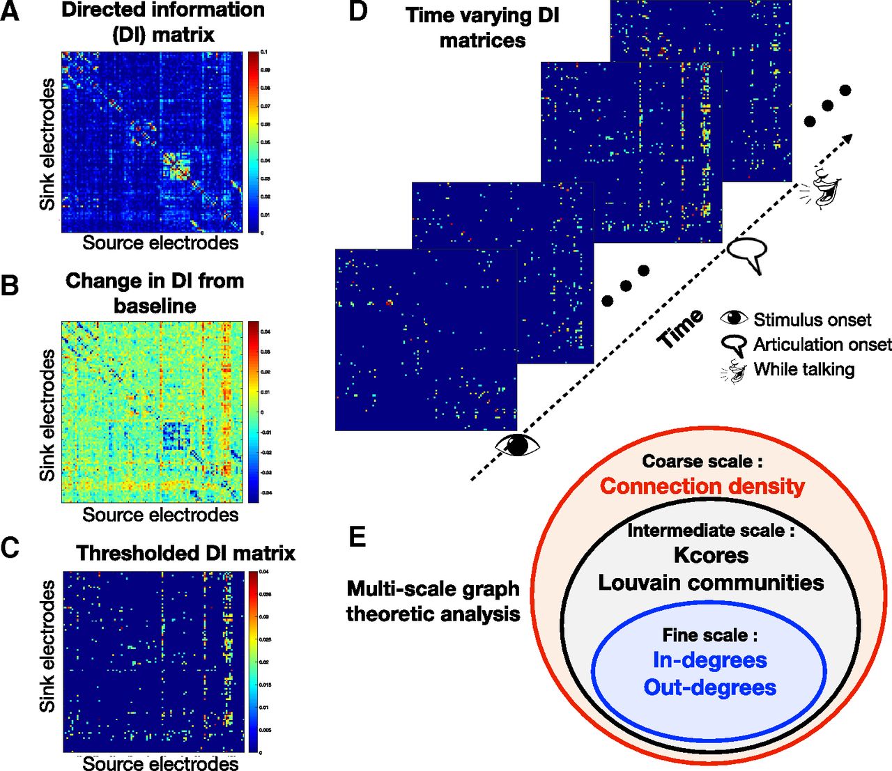
A, DI matrix in a window; x- and y-axes are the electrodes and the  element represents DI from the
  to the
  electrode. B, The DI matrix relative to the baseline (“change in DI” matrix) is obtained by subtracting the baseline DI matrix from the DI matrix of that window. C, The thresholded DI matrix, which only retains the top positive increases in DI, based on a threshold value T (described in Materials and Methods). D, W = 52 “increase in DI” matrices were generated per patient. E, Multiscale graph analysis.
Coarse scale, connection density
A patient with M electrodes has W thresholded adjacency matrices Aw, for each window w, of size M × M. The connection density of each matrix defined as the ratio of the number of connections (non-zero values) in the adjacency matrix, to the total number of possible connections M2-M. The results of one patient’s connection density versus W time windows is shown in Figure 5A.
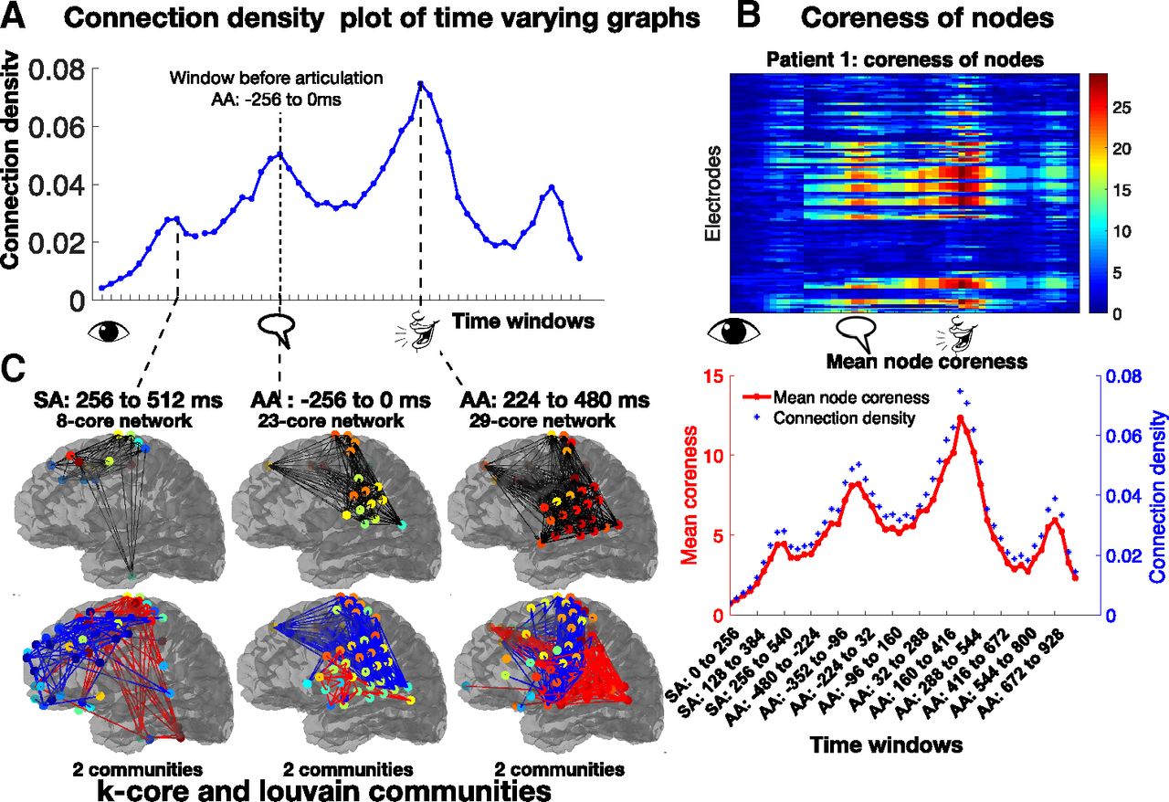
A, Connection densities vary smoothly across time windows, with a local maximum occurring before articulation. B, Coreness of nodes heatmap identifies sets of nodes in the brain related to changes in connection density. The average coreness across nodes (shown in red below the heatmap), provides the same information as the coarse scale metric (in blue). C, The first row shows the maximal k-core network in windows where peaks were found in the coarse metric. Connections are shown in black lines. The max k-core network is a very strongly interconnected core of the graph. The second row shows the results of the Louvain analysis. The colors of directed lines only indicate that the nodes belong to the same community. Significant communities, Bonferroni corrected p < 0.05 are shown.
Intermediate scale, coreness of nodes
K-cores analysis (Hagmann et al., 2008; Modha and Singh, 2010) is an intermediate scale graph theoretic metric, calculated using directed binarized graphs (Rubinov and Sporns, 2010a,b). K-cores of a graph are a set of connected components that remain, after all vertices of degree less than k have been removed, in an iterative manner. Coreness of node quantifies the highest k-core network a given node belongs to (Fig. 3A). The coreness values of the nodes were evaluated as follows (Shin et al., 2016): First, the 1-core network was identified by finding the isolated 0-degree nodes of the graph. These nodes were given a coreness value of 0, and then deleted from the network to reveal the 1-core network. Next, the 2-core network was identified, and the nodes deleted at this step were given the coreness value of 1. This process was repeated until every node was given a coreness value, until the largest k-core subnetwork of each graph Gw was found. The coreness of all nodes of a patient versus time windows has been plotted as a heatmap, as shown in Figure 5B. This revealed which set of nodes were involved in highly connected subnetworks, and in which time windows this occurred.
Intermediate scale, Louvain algorithm: maximizing modularity
The Louvain algorithm (Reichardt and Bornholdt, 2006; Blondel et al., 2008; Ronhovde and Nussinov, 2009; Sun et al., 2009) is a fast, heuristic, agglomerative community detection algorithm, that finds the optimal partition structure of the nodes into communities, by maximizing a measure of partition quality; the modularity index Q (Newman and Girvan, 2004), example in Figure 3B. The Louvain algorithm in this work used an adapted modularity index suitable for directed weighted networks (Rubinov and Sporns, 2010a,b, 2011). It uses a greedy optimization phase which randomly selects the starting node, leads to an inherent variability of the Louvain algorithm. To overcome this, consensus clustering was done (Rubinov and Sporns, 2011; Lancichinetti and Fortunato, 2012; Dwyer et al., 2014), where the algorithm was run R = 100 times, and an R × R module allegiance matrix (Bassett et al., 2013, 2015) was created. The community detection algorithm was then run for a second time on this module allegiance matrix, which revealed the most robust partition of the data (Lancichinetti and Fortunato, 2012). The number of communities in each graph was determined by the output of the algorithm. The Louvain communities in three windows for a patient are shown in Figure 5C.
Fine scale, in-degrees and out-degrees of nodes
For a node  , in-degrees
  and out-degrees
  provide a fine grained view of the graph structure, for time windows
  . For weighted, directed networks, in-degrees of a node is defined as the sum of the weights of the edges entering that node.
  . Similarly, out-degrees of a node is defined as the sum of the weights of the edges leaving that node.
  . In-degrees is a measure of the sink strength of the nodes, while out-degrees measures source strength (Fig. 3C). The significant correlations between in-degrees and power, and out-degrees and power for all patients are shown in Figure 6 and Figure 7.

A, An inf-frontal gyrus pars opercularis electrode from patient 1, that shows positive correlation between hγ power and the network features. B, A negatively correlated orbital frontal cortex from patient 6. The coreness of nodes can be seen as a combined effect of in and out degrees. A detailed figure that shows the correlation coefficient of in/out degrees with other frequency bands is shown in Extended Data Figures 6-1, 6-2. A pictorial understanding of how in/out degrees correlates with power is shown in Extended Data Figure 6-3. R represents the correlation coefficient.

Every three-ring electrode on the brain denotes the correlation coefficient value of three feature spaces with power. The significant correlation coefficient of in-degrees and hγ power time-series are shown in the innermost circle, the correlation coefficient of out-degrees with power is denoted by the color of the middle ring, while the outer ring for each electrode’s color denotes the correlation coefficient of coreness of nodes with power. The absence of color in the outer ring, or the absence of either the middle or inner ring, denotes the lack of significant correlation in that electrode, with that feature space. This figure denotes the correlation coefficient calculated using the entire time-series, SA and AA time windows considered separately are shown in Extended Data Figure 7-1. The bar plot to the right shows the average percentage of electrodes that showed significant correlation for each feature space, after correcting for multiple comparisons (FDR, p < 0.05 for each feature space, per patient). It can be noted that most electrodes’ feature spaces show correlation in the same direction. Across patients, more electrodes have significant correlation of coreness of nodes feature space with power, than the other two feature spaces.
Relationship between network features and power
The relationship between network features (coreness of nodes, in-degrees, and out-degrees) and power of each was evaluated to understand how network features and power could be related. We conducted the following analyses, which are summarized in the results. We analyzed positive and negative correlations of network features and hγ power, results shown in Figure 6. We evaluated correlations between in-degrees, out-degrees with power in five frequency bands (hγ, γ, β, α, and θ), and demonstrated the relationships between the frequencies and the network features, results shown in Extended Data Figures 6-1, 6-2. An intuitive understanding of how in/out degrees correlate with power is shown in Extended Data Figure 6-3. Evaluated correlations between coreness of nodes, in-degrees, out-degrees with hγ power, for all time windows (SA + AA; results in Fig. 7). Evaluated correlations between coreness of nodes, in-degrees, out-degrees with hγ power, for time windows SA and AA separately, since the processes underlying SA and AA windows could be different (results in Extended Data Fig. 7-1).
With an understanding of how network features are related to power, we then evaluate whether network features provide additional information to the language process, compared with power alone, using data from DCS.
Direct cortical stimulation
DCS was used to map brain function before surgeries, wherein targeted transient dysfunction was induced via electrical stimulation, providing causal functional inference. DCS revealed which node-pairs were PN positive and language negative for brain regions, in the following manner. In order to map brain function using DCS, a patient performed three tasks: a PN task, an auditory repetition task, and an auditory naming task. During each task, a pair of electrodes (node-pair) were stimulated with an electric current. If the stimulation disrupted the PN task, then that node-pair was considered PN positive. Each task was tested separately. If the current stimulation did not disrupt any of the three language tasks tested individually, then that node-pair was considered to be language negative. DCS caused a reversible temporary lesion, and allowed the doctor to assess the importance of that node-pair for brain resection. Note: The PN task for DCS is different from the PN task done for analysis using NetDI for research purposes.
Comparison of network/power features using classification of node-pairs
The DCS data labels: PN positive or language negative for node-pairs were considered as ground truth. Using standard machine-learning classifiers and a training and testing paradigm, the accuracy of classification of node-pairs were compared using various power and network feature spaces, namely, (1) hγ power of the node-pairs, (2) in-degrees, (3) out-degrees, (4) both in-out degrees (5) coreness of nodes; and using a combined network and power feature space: (6) in-degrees and power features, (7) out-degrees and power, (8) combined in/out degrees and power feature space, and (9) combined coreness of nodes and power. Multiple classifiers were used to eliminate bias in the results because of a particular classifier. A comparison of classification accuracy across these nine feature spaces would reveal insight into which feature space had higher discriminability to classify between the PN positive and language negative node-pairs. The total number of labeled node-pairs (n), and the length of each feature space (p) together form an n × p matrix, (n < p), which is used for classification. For example, the power feature space was created by taking the power time series (from 52 windows) for each node of the node-pair, concatenating them to produce a vector of length 104 for that node-pair. Every DCS node-pair provided two data samples for classification, as features from node-pairs could be concatenated in two ways. Specifically, each DCS node-pair was used to generated another labeled node-pair by reversing the order of the nodes in which the features were concatenated, thus doubling our available labeled node-pairs. Thus, in this work, the effective n for classification varied between 26 and 46 for the patients, while p varied between 104 and 312, based on the feature space considered. The number of labeled node-pairs were sufficient to estimate classification accuracies with a 95% confidence interval. For each feature space, 5-fold cross validation was performed, with repeated random splits of the data (Varoquaux et al., 2017), keeping the training and test sets stratified, to have a balanced split among the two classes. The results are averaged over the test sets. Remark: Our previous efforts with using the original DCS node-pairs had insufficient samples for 5-fold cross validation and confidence interval estimation. Classification accuracies found using the leave-one-out cross-validation methodology were similar to the results and trends among feature spaces presented in this paper, but did not have additional statistics provided here.
A brief note on notation: TP(FP) stands for true(false) positives, TN(FN) for true(false) negatives. True positive rate (TPR), also known as sensitivity or recall is given by  . True negative rate (TNR) is also called specificity or selectivity is
  . Precision is given by
  . For all patients, the number of PN positive and language negative node-pairs were not equal, so the balanced accuracy metric was used, by normalizing true positive and true negative predictions. Balanced accuracy
  .
.
Statistical analysis
Significance of network-based measures were evaluated using controls and statistical tests. The statistical significance of the Louvain communities in each graph was calculated using non-parametric permutation testing (Park et al., 2009) by randomly permuting the community labels assigned to the nodes 5000 times. The final communities reported were Bonferroni corrected p < 0.05. The network measures in-degrees, out-degrees, and coreness of nodes were correlated with the power responses, the significant correlations,  , FDR corrected were reported. All comparisons of classification accuracy among different feature spaces were reported with statistical significance for p < 0.05, using t tests, also FDR corrected for multiple comparisons, among feature spaces.
Code and software
The NetDI analysis was performed in MATLAB 2014b, while the DCS classification analysis was done using Python’s Sci-kit learn machine learning toolbox (Pedregosa et al., 2011) in Jupyter notebooks. Python version 3.7 was used. Code used to develop the NetDI analysis and the classification analysis based on DCS are provided online at https://github.com/ysudha/NetDI.
Results
Multiscale network analysis
The brain processes span multiple resolutions, and hence it was important to analyze the dynamics at multiple scales. The first step of NetDI was to estimate causal information flow between brain regions. Pairwise bias-corrected DI (see Materials and Methods) between all pairs of electrodes were calculated for each window  (Fig. 4A), followed by a baseline normalization of DI (Fig. 4B) and thresholding (Fig. 4C). Each resulting DI matrix was interpreted as an adjacency matrix of a graph, whose nodes are fixed electrodes, and the edges between the nodes are based on the increase in DI between them. The second step of NetDI was to obtain spatiotemporal dynamics from the resulting time-series of graphs. Graph theoretic tools at coarse, intermediate, and fine scales of resolutions (Fig. 3) were then used to analyze the graphs.
Connection density is a coarse scale metric, that provided a single number per graph; the plot for patient 1 is shown in Figure 5A. The connection density plot had a temporal pattern, with local temporal maxima (peaks). One peak occurred exactly at the window immediately preceding articulation (AA: –256 to 0 ms). The timing of the peak suggests that the connections in that window represent “local decisions” being made. By extension, the peak in the SA windows at SA: 256 to 512 ms could relate to word identification, and the peak after articulation at AA: 224 to 480 ms may relate to a brain process that occurs while the patient is still speaking.
Coreness of nodes (Hagmann et al., 2008) is an intermediate scale metric, that was plotted as a heatmap in Figure 5B. It spatially identified the nodes that belonged to the higher cores, and were thus more central to the network, quantified by their coreness values. The Louvain community detection algorithm (Newman and Girvan, 2004; Blondel et al., 2008; Rubinov and Sporns, 2011) optimally partitioned the graph into communities or clusters of nodes, in each time window, revealing insight into interconnectivity among brain regions and dynamical properties of these connectivity. The communities in the temporal peaks identified by the coarse scale metric are shown in Figure 5C, and the brain regions most connected in each local decision were identified.
Fine scale granular information about the graph were obtained at the node level. The in-degrees and out-degrees revealed the sink and source strength of the nodes, in each window.
Correlations between  power and network features of nodes

To understand the network correlates of the power, we investigated relationships between the network measures: coreness values, in-degrees, out-degrees, and the local power responses. Across multiple nodes, all three network features were found to be correlated with the hγ power. Brain regions with positive, and negative significant correlations were found, example nodes are shown in Figure 6A,B, while Extended Data Figure 6-3 shows the evolution of the in-degrees and out-degrees to obtain an intuitive understanding of these correlations. Many negative correlations, especially those in the frontal brain regions, were dominated by sharp decreases in hγ power in the SA windows that coincided with an increase in the node’s coreness value.
Figure 7 illustrates the locations of the statistically significant Spearman’s correlations between the three network measures and the hγ power, with 49% of nodes showing correlations with coreness, 43.3% with in-degrees and 34.9% with out-degrees. Most electrodes showed correlations in the “same direction” for all three network features, except for a total of 5 electrodes out of 711 total electrodes for all patients. This analysis was also repeated considering just the SA, and AA windows separately, as different processes govern these two time windows (Extended Data Fig. 7-1). As expected, some brain regions do show opposite directions of correlations in these windows, yet, the overall trend of maximum number of correlations with coreness feature space remains the same.
Finally, we examined the correlation of network features with other narrowband frequency power spectrums, as it is well known that powers in different bands are themselves correlated. The results of correlation of the network features with powers in other bands, particularly the θ (4–8 Hz), α (8–13 Hz), β (13–30 Hz), and γ (30–60 Hz) bands in addition to the hγ band (hγ: 60–150 Hz; details in Extended Data Figs. 6-1, 6-2), reveal that it is indeed the case that powers in different frequency bands are themselves related. The electrodes that showed strong positive correlations with hγ power, also showed strong negative correlations with θ, α, and β power. The significantly correlated electrodes were mostly in pars opercularis and triangularis regions of the left inferior frontal gyrus, also called Broca’s region; as well as motor cortex and superior temporal gyrus (STG) regions.
The results of the correlation analysis indicate that the centrality of a node given by its coreness value is related to the power responses of the node. The results indicate that both increases and decreases in power seem related to how central the node is in the network.
DCS data
DCS is the current gold standard in mapping brain function onto the cortex, before brain resection surgeries. DCS informs the neurosurgeon of language critical areas, to estimate the risk, and potential outcome of the brain resection surgeries. DCS was performed on the same patients as those in whom ECoG data were analyzed, to map out language-specific brain regions before surgery. The DCS data identified which node-pairs were PN positive or language negative, after excluding nodes that had epileptic activity (Fig. 8). DCS data from all seven patients were considered, but only four patients had sufficient DCS node-pairs for classification analysis. Details of all node-pair labels for all patients is given in Table 2.
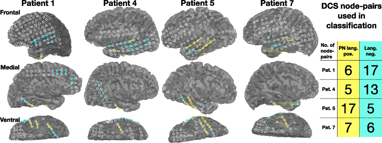
Location of PN positive and language negative node-pairs obtained after DCS. These node-pairs are used as ground truth labels for classification.
Node-pair labels obtained from DCS for all patients
Classification results using DCS data as the ground truth
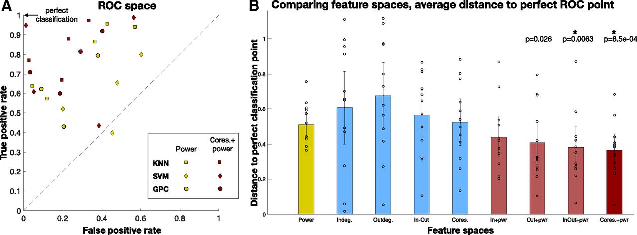
A comparison of classification accuracy across the nine feature spaces was done to reveal insight into which feature space had greater classification accuracy between the PN positive and language negative node-pairs. Three classifiers were used: kNN classifier (Bentley, 1975), linear support vector machine (SVM) classifier (Fan et al., 2008), and the Gaussian process classifier (GPC; Rasmussen, 2003; Rasmussen and Nickisch, 2010) for each of the nine feature spaces, using Python’s Sci-kit learn machine learning toolbox (Pedregosa et al., 2011), to classify between PN positive and language negative node-pairs. Five-fold cross validation was performed with stratified training and test splits, to ensure that classes were balanced. Furthermore, to increase the number of splits while keeping a fixed ratio between training and test set size, repeated random splits of the data were performed 100 times (Varoquaux et al., 2017). The balanced accuracy results of the three classifiers across all test sets are shown in Table 3, with their 95% confidence intervals. Figure 9 summarizes the results from the table, which shows the balanced classification accuracy for each feature space. While all four network features show greater accuracy than power, it is not statistically significantly greater than power. Combined power and network features had higher accuracy; with the highest accuracy feature space being “coreness and power,” statistically significantly greater accuracy than power (p = 0.0039, t test, significant after FDR correction). To combine results across patients and classifiers, every classifier result was plotted in the ROC space, which plots the TPR versus the FPR. The average distance of classification based on each feature space for all patients and classifiers, to the perfect classification point (TPR = 1, FPR = 0) revealed which feature space had the best classification in the ROC space, shown in Figure 10. The results show that across patients, the feature space coreness+power was closest to perfect classification, significantly closer than the power feature space ( , t test, FDR corrected).
Balanced accuracy results (%) for binary classification between PN positive and language negative node-pairs
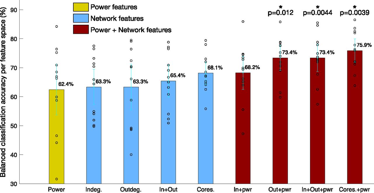
Comparison of binary classification accuracy between PN positive and language negative node-pairs using different feature spaces. The average accuracy in each feature space across all classifiers and patients are shown, with their 95% confidence intervals. While classification accuracy is greater when using network features alone than using the power, it is not significantly greater. However, combining network features and power, “out-degrees+power,” “both in-out degrees+power,” and “coreness+power” perform significantly better than power alone, with “coreness+power” being the best feature space. * indicates p < 0.05, the cyan lines indicate the 95% confidence interval, while the black dots are the original data points.

A, Each classifier was plotted in the ROC space. TPR = 1, FPR = 0 is the perfect classification point in this space. There are four points for each colored shape, for four patients. B, The average L2 distance to the perfect classification point, for each feature space is shown in the bar plot, with the 95% confidence interval. Coreness+power feature space is the closest to perfect classification, across all patients, and accounting for classifier variability. Feature spaces “in-out degrees+power” and “coreness+power” perform significantly better than power alone ( , t test, FDR corrected).
Extended Data Table 3-1
Sensitivity (recall or TPR), specificity (selectivity or TNR), precision for kNN classification Download Table 3-1, DOC file.
Extended Data Table 3-2
Sensitivity (recall or TPR), specificity (selectivity or TNR), precision for SVM classification Download Table 3-2, DOC file.
Extended Data Table 3-3
Sensitivity (recall or TPR), specificity (selectivity or TNR), precision for Gaussian process classification Download Table 3-3, ZIP file.
Finally, we report the sensitivity (also called recall or TPR), specificity (selectivity or TNR), and precision along with their 95% confidence interval for each classifier in the Extended Data Tables 3-1, 3-2, 3-3. The results clearly show greater classification accuracy from a combined power and network feature space, with the best performing feature space being coreness values+power.
Discussion
Of all the millions of species inhabiting our planet, we Homo sapiens are uniquely gifted in our expressive power through language. We effortlessly articulate two to three words per second in fluent speech, yet this deceptively simple task is a highly complex multistage process in our brains (Indefrey and Levelt, 2004; Hickok and Poeppel, 2007). Unfortunately, when disease and brain damage affect such an intricate speech language system, it causes a variety of disorders in millions of people, many of which remain irremediable. Decades of research have greatly enhanced our understanding of these language processes (Dell et al., 1999; Indefrey and Levelt, 2004; Riès et al., 2013; Munding et al., 2016), yet, there exist gaps in our knowledge, particularly in understanding the underlying neural dynamics (Medaglia et al., 2015; Herbet and Duffau, 2020).
Historically, language has been analyzed in a localized manner with a goal of associating cognitive processes to specific brain regions, evidenced by regions’ activation profiles. Recently, language has begun to be studied as a network phenomenon (Bassett and Bullmore, 2009; Fedorenko and Thompson-Schill, 2014; Braun et al., 2015; Forseth et al., 2018; Saravani et al., 2019; Skeide and Friederici, 2016), as it has been theorized that network properties provide greater understanding of the neurobiology of language (Medaglia et al., 2015; Chai et al., 2016).
In prior work, cognitive flexibility is hypothesized as dynamic integration between brain areas in Braun et al. (2015), while Bassett et al. (2015) address the hypothesis that sets of brain regions preferentially interact during a task, and if such interactions differ with learning. Other studies speculate that syntactic processing is distributed across a large ensemble of brain regions (Blank et al., 2016; Xiong and Newman, 2021). All these studies are based on fMRI data. There is an increased focus on studies based on multiscale (Betzel and Bassett, 2017; Domenico, 2017) and modular brain functions (Betzel et al., 2017; Martinet et al., 2020). A review of contributions of network science to cognitive neuroscience using neuroimaging data are in Medaglia et al. (2015), while Herbet and Duffau (2020) is a comprehensive review on the concept of network theory of brain functions. Our work quantitatively evaluated network dynamics using both recording and disruption evidence from ECoG and DCS data.
We interpret “network phenomenon” as multiple physical brain regions, that functionally connect together to subserve a cognitive brain function; and they reconfigure connections as processing goes forward, similar to Salehi et al. (2020). To illustrate with an example; for decades, Broca’s area (inferior frontal regions) was thought to be primarily responsible for speech articulatory processes. While Broca’s area has now been shown to be involved in other cognitive processes as well (Hagoort, 2014; Fedorenko and Blank, 2020); our network view assumes that Broca’s area in conjunction with other brain regions forms a network, and the brain network is responsible for speech articulation.
In this study, we quantitatively measured network dynamics in PN, by assessing the hypotheses: Are different cognitive functions being supported by different network states, or by single regions? In other words, are network measures of brain regions or power profiles of a single region are more predictive of identifying critical language areas?
A majority of previous works using ECoG data have shown that hγ power is a great indicator of local task activity (Salmelin et al., 1994; Crone et al., 2001; Edwards et al., 2005; Towle et al., 2008; Cogan et al., 2014; Conner et al., 2014; Flinker et al., 2015; Riès et al., 2017). Our data analysis from the PN task from seven patients validated the same phenomenon. Similar to previous work (Kadipasaoglu et al., 2014; Flinker et al., 2015), for each trial, we found strong increases in hγ power in the visual cortex, aligned to the stimulus onset, and a strong increase in hγ aligned to the start of articulation time in the pre-motor cortex regions. Furthermore, a strong increase in hγ in visual cortex in SA windows was accompanied by strong decreases in hγ power in some frontal regions, for all patients. Such patterns of power activations and deactivations were seen in many brain regions during the task. The NetDI methodology allowed us to obtain network dynamics among these brain regions, and we asked the following questions: (1) Is there a relation between the network measures and the local power responses? (2) Do the network measures contain any additional information about the language processes, compared with power? The answers to these questions are indicative of the original hypothesis, about whether cognitive functions are supported by brain networks, or local brain regions. To answer the first question, we investigated relationships between hγ and the network measures, to understand the various aspects of the relationships. To answer the second question, we performed a classification analysis between PN positive and language negative node-pairs, considered as ground truth, using DCS data (Ojemann et al., 1989; Sinai et al., 2005), for the same set of patients for whom the NetDI analysis was done.
In order to understand the network basis of power responses, we developed a graph theoretic framework NetDI, to discern the spatiotemporal brain dynamics underlying language. DI provided a robust information theoretic measure of causality, even if the underlying data were nonlinear. A multiscale graph theoretic analysis revealed network properties of the process at various scales. The coarse scale analysis revealed task related peaks in temporal dynamics conjectured to be local processing “stages” in the brain, because of their strong alignment with task activities. These stages could correspond with separable cognitive processes that are thought to be invoked during speech production (Levelt, 1989; Salmelin et al., 1994). At an intermediate scale, k-cores and the Louvain analysis provided alternate spatiotemporal views of the process. K-cores uncovered the highly interconnected innermost core of the network, providing “coreness values” for each node, as a measure of centrality of the node in the network. The Louvain analysis revealed a distributed overlapping set of communities with very strong interconnectivity within each community, consistent with recent suggestions toward interactive networks in Betzel and Bassett (2017), Saravani et al. (2019), and Martinet et al. (2020). The fine scale analysis revealed the out-degrees (source strength) and in-degrees (sink strength) of the nodes, time-varying network measures that provide additional insight into the language process.
Armed with these network measures, we sought to understand whether there existed a relation between the network measures and the local power responses. All three network features, coreness values, in-degrees and out-degrees were significantly correlated with the hγ power, with most electrodes showing positive and negative correlations with coreness values. The network measure coreness of nodes values is a measure of the centrality of the node, and typically depends on both in-degrees and out-degrees. Our results align with prior work that indicated coreness of nodes as a good measure of a node’s influence in the network (Kitsak et al., 2010; Pei et al., 2014; Shin et al., 2016). In Xiong and Newman (2021), language processing was found to be supported by activation of both core networks, and periphery brain regions. Our results show that a region’s coreness and power features contain different information about the language process. This is substantiated by the fact that there were both positive and negative correlations, which could indicate different processes where the centrality of the node was related to either the increase or decrease in hγ power. Furthermore, differences in correlations between SA and AA windows also existed, along with different fine-scale measures that drove the correlations. It seems that the information content of in-degrees, out-degrees and coreness values are related to hγ power, but not equivalent.
In order to quantitatively verify whether the network measures contain additional information from power, the data from DCS were used to classify language areas as critical to processing (PN positive) or not (language negative) using feature spaces consisting of power, network measures and a combination of power and network feature spaces. The classification results across patients and multiple classifiers indicate superior classification of combined network and power features compared with power alone. The feature space consisting of coreness of nodes and power emerged as the best classifier, thus indicating that the centrality of the node in the network is an important feature for understanding language dynamics. This confirms the hypothesis that network features do contain provide novel information about the language process beyond information given by power. Our results agree with other studies like (Jiang et al., 2020; Salehi et al., 2020) where functional networks dynamically are hypothesized to reconfigure based on cognitive states, in an individualized manner. Extensive recent work in aphasia studies suggest that patients with seemingly different lesion locations could experience similar impairments, probably because the lesions affect a broad cortical network needed for the language task (Fridriksson et al., 2018). Our results provide further evidence that the centrality of the brain region has a critical role to play in the language system, beyond the local processing of the region.
Future research directions
(1) The hγ power in ECoG data are a component of the local field potential signal, which is inherently ambiguous because of contributions from multiple sources like synaptic inputs, spikes and volume conduction, making them harder to interpret. Further studies could elaborate on the various subcomponents of the network basis of power. Furthermore, it would be interesting to study the differences between the various frequency bands, similar to Lam et al. (2016), in terms of discriminability between language critical and language negative areas, to understand spectral components of the language process.
(2) The examination of Louvain communities indicates that the PN positive brain regions had strong connectivity with distant brain regions. Within the Louvain communities, the was a lack of connections between the node-pairs themselves, the nodes involved in PN positive areas were instead connected with distant brain regions. We speculate that DCS did not just disrupt a local process, but rather disconnected the local brain region from downstream brain regions, however further studies need to be done to prove or disprove that.
(3) In future work, NetDI could be used to improve pre-surgical DCS language mapping in patients (Szelényi et al., 2007). DCS has some unpleasant side-effects, it sometimes induces seizures and has after-discharge effects, so the doctors would prefer to test only as many regions as is essential for clinical mapping. Network and power measures can be found for all nodes, from experiments before performing DCS. Given a few ground truth node-pairs, the corresponding network measures could be used as training data to identify other potential language positive and negative areas, to guide doctors in making DCS more clinically efficient.
(4) This work is important in understanding why certain focal brain lesions cause widespread disruption of the networks of the brain (Gratton et al., 2012; Fridriksson et al., 2018). Overall, NetDI has the potential to relate brain cognitive theories of language with the neural connectivity patterns, and can validate cognitive theories of language (Dell, 1988; Dell et al., 1999; Bassett and Bullmore, 2009; Salehi et al., 2020).
Extended Data Figure 6-1
A matrix representation of correlation coefficients of in and out degrees with powers in five frequency bands are shown for each of the seven patients. Rows of all matrices are electrodes grouped by brain region, and there are 10 columns for each patient. First two columns are correlation coefficient of in-degrees and out-degrees with hγ power (60–200 Hz), next two columns are in/out-degrees with γ power (30–60 Hz), next two columns are correlation coefficient of in/out-degrees β power (13–30 Hz), next two columns are correlation coefficient of in/out-degrees α power (8–13 Hz), while the last two columns are with θ power (4–8 Hz). It can be observed that while the electrode coverage of all the patients is different, there exist similar trends of high positive correlation with hγ power and negative correlation with the θ power, particularly in language-related brain regions. The brain regions are labeled with numbers and are enumerated in Extended Data Figure 6-2. The exact number of electrodes that were positively and negatively correlated for in-degrees and out-degrees are also shown, and more electrodes were found to be negatively correlated with out-degrees than in-degrees, while greater number of electrodes are positively correlated with in-degrees than out-degrees. Download Figure 6-1, EPS file.
Extended Data Figure 6-2
Table depicting the brain regions and number of recording electrodes in each region for all patients. Download Figure 6-2, TEX file.
Extended Data Figure 6-3
A, A positively correlated occipital-temporal-lateral-fusiform-gyrus electrode from patient 5. B, A negatively correlated Inf-temporal electrode from patient 5. The colors of the nodes in A, B represent the power in the window, while the dark blue lines are in-degrees to the node, and the light blue lines are the out-degrees. These figures demonstrate that coreness of nodes is due to the combined effect of in and out degrees and provide a pictorial understanding of how in/out degrees correlates with power. Download Figure 6-3, EPS file.
Extended Data Figure 7-1
Every three-ring electrode on the brain denotes the correlation coefficient value of three feature spaces with power. The significant correlation coefficient of in-degrees and hγ power time-series are shown in the innermost circle, the correlation coefficient of out-degrees with power is denoted by the color of the middle ring, while the outer ring for each electrode’s color denotes the correlation coefficient of coreness of nodes with power. The absence of color in the outer ring, or the absence of either the middle or inner ring denotes the lack of significant correlation in that electrode, with that feature space. The first row denotes the correlation coefficient calculated using the entire time-series, and is the same as the main figure in the paper. The second row shows the correlation coefficient of the three feature spaces with power, when only the SA time windows are considered, while the third row shows the correlation coefficient when only the AA windows are considered. The bar plots to the right denote the average percentage of electrodes that showed significant correlation for each feature space, after correcting for multiple comparisons (FDR, p < 0.05 for each feature space, per patient). It can be noted that most electrodes’ feature spaces show correlation in the same direction. There are electrodes where the correlation in SA and AA are in the opposite directions, and are canceled out in the combined SA+AA correlation space. Overall, more electrodes have significant correlation of coreness of nodes feature space with power, than the other two feature spaces, in all three various time-window considerations. Download Figure 7-1, EPS file.
Acknowledgments
Acknowledgements: We thank Prof. Simon Fischer-Baum for reviewing this manuscript and providing invaluable comments. We also thank Cristian Donos, Patrick Rollo, Oscar Woolnough, and Eleonora Bartoli for help with generating brain plots, thoughtful comments and discussions.
Footnotes
The authors declare no competing financial interests.
This work was supported by the National Science Foundation Integrative Graduate Education and Research Traineeship Award 1533688 and the National Institute on Deafness and Other Communication Disorders Grant F30DC017083.
This is an open-access article distributed under the terms of the Creative Commons Attribution 4.0 International license, which permits unrestricted use, distribution and reproduction in any medium provided that the original work is properly attributed.
References
In this issue


