

Article Figures & Data
Figures
- Figure 1.
Experiment 1, behavior. A, Illustration of a successful trial in experiment 1 (n = 14). Participants were instructed to wait for the go signal and then to reach for the goal within 0.6 to 0.8 s of the go signal. Feedback about movement timing was provided to encourage participants to adjust their movement speed, but all trials were included in the dataset. B, Hand paths from all participants for the first FF trial (top) and the FF trial number 20 (bottom), were selected to illustrate the change in online control. CCW and CW FF trials are depicted in blue and red, respectively. The black traces (baseline) are randomly selected trials from each participant. Maximum deviation in the direction of the FF (Max.) and the maximum target overshoot (Osh.) are illustrated. C, Maximum hand path deviation for CCW and CW FFs across trials. The dashed traces illustrate the non-significant exponential fits. D, Maximum target overshoot across FF trials. Solid traces indicate significant exponential decay. Shaded blue and red areas around the means indicate the SEM across participants. E, Illustration of the after effect. Baseline trials were categorized dependent on whether they were preceded by CCW or CW FFs, or by at least three baseline trials. F, Continuous traces of x-coordinate as a function of time and extraction at the moment of peak lateral hand force (dots). Error bars at 300 ms illustrate the SEM across participants. G, individual averages of lateral hand coordinate (gray), and group averages (mean ± SEM), after subtracting each individual’s grand mean for illustration). One (two) star(s) indicate significant difference at the level p < 0.05 (p < 0.01) based on paired t test, adjusted for multiple comparison with Bonferroni correction. NS, not significant.
- Figure 2.
Improvement in online corrections. A, Lateral perturbation force (dashed/light) and measured force (solid/dark) as a function of time for the first FF trial in each direction. B, Same as panel a for the last perturbation trial. Shaded areas represent 1 SEM across participants (n = 14) with the same color code as in Figure 1. Note that each FF induced a reaction force with opposite sign, thus the perturbation force was multiplied by –1 for illustration. The reduction in peak end force is highlighted with the black arrows. C, Peak end force across FF trials (mean ± SEM). The solid traces show the significant exponential decay (p < 0.005). D, Correlation between the commanded force and the measured force during the time interval corresponding to the gray rectangle in panel A (100–700 ms). The correlations were averaged across participants; the shaded area represents 1 SEM. The significant linear regression of the correlations across blocks is illustrated.
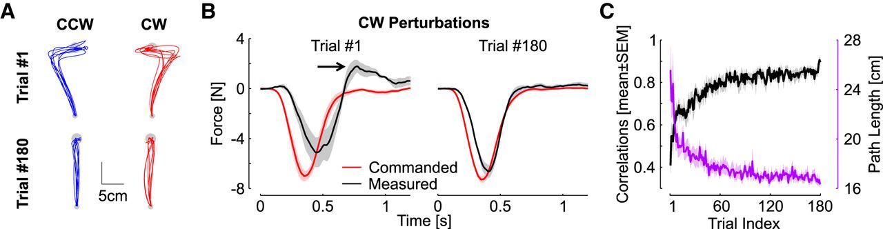
- Figure 3.
Control experiment. A, Hand paths of the first and last trials for each perturbation direction. Displays are individual movements corresponding to one trace for each participant. B, Commanded and measured forces for the first and last trials. Shaded areas are 1 SEM across participants (n = 8). C, Black: correlations between commanded and measured forces across trials. Purple: path length across trials (mean ± SEM across participants).
- Figure 4.
Experiment 2. Behavior. A–C, Illustration of the FF trials and behavior as reported in Figure 1B–D. D, correlations between the commanded force and the measured force across FF trials similar to Figure 2D. E, Average hand traces from experiment 2 for trials with a via-point with the same color code as in experiment 1 (black: null-field, red: CW, blue: CCW). For all trials, the second portion of the reach, from the via-point to the goal, was performed without FF (FF Off). F, Average x-coordinate as a function of time across participants (n = 14). Shaded areas represent 1 SEM across participants. The gray rectangle illustrates the approximate amount of time spent within the via-point. Observe the displacement following the via-point in the opposite direction as the perturbation-related movement. G, Illustration of the trial-by-trial extraction of parameters on five randomly selected trials from one participant. The FF was turned off when the hand speed dropped below 3 cm/s (dashed trace). The parameters extracted were the lateral hand velocity at the moment of the hand speed minimum (squares), and the lateral hand velocity at the moment of the second hand speed maximum (open discs). H, Lateral hand velocity at the moment of hand speed minimum or at the moment of the second hand speed maximum averaged across trials for each participant (gray dots), and averaged across participants (blue, black, and red, mean ± SEM). Individual means across the three trial types were subtracted from the data for illustration purpose. The stars represent significant pair-wise differences at the level p < 0.005 with Bonferroni correction for multiple comparisons. NS, not significant.
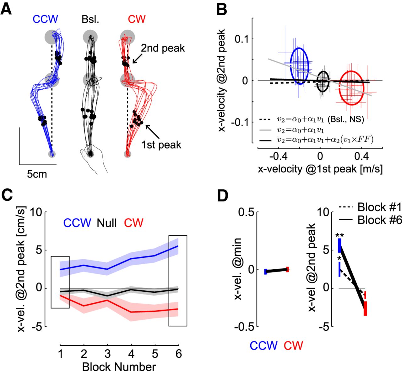
- Figure 5.
Kinematics after the via-point. A, Extracted parameters. The lateral velocity (x-direction) was extracted at the moment of the first and second peaks of hand speed prior and after the via-point, respectively (dots and arrows). Vertical dashed lines were added to highlight the systematic deviation opposite to the perturbation during FF trials. We selected 10 traces randomly per condition from one representative participant. B, Lateral velocity at the second peak as a function of the lateral velocity at the first peak. Crosses are mean ± SD across trials for each participant (n = 14). Dispersion ellipses illustrate 1 SD along the main variance axes (all trials pooled together). The three statistical models are illustrated with thick lines: baseline trials only (not significant), all trials (gray), and all trials with categories as factor (black plus average of the categories represented with the ellipses). The thin black line is the value of 0 displayed for illustration. Participants were included as random factor. C, Lateral hand velocity measured at the second peak hand speed following CCW and CW force-fields (red and blue, respectively), and baseline trials (black) across blocks. Data are from 11 participants who completed successful trials in each block. The insets highlight the first and last block. D, Group data mean ± SEM in the 1st and 6th block for the lateral hand velocities at the minimum and at the second peak (n = 11 in both cases). Observe the two different scales. One (two) star(s) highlight significant difference based on paired t test at the level p < 0.05 (p < 0.005).
- Figure 6.
Model simulations. A, Schematic illustration of an adaptive controller: sensory feedback is used to estimate both the state of the system and the model, which in turn updates the controller and estimator online. The solid arrows represent the parametric state-feedback control loop, and the dashed arrows represent the real-time learning and update of model parameters. B, Reproduction of a standard learning experiment (hand paths and maximum lateral deviation across trials), with mirror-image catch trials (ct), and unlearning following the catch trials (difference between ct-1 and ct+1). The trial-by-trial changes were reproduced with online computations exclusively (Thoroughman and Shadmehr, 2000). C, left, Simulation of the results from experiment 1 with three distinct values of online learning rate ( γ : 0.1 in black, 0.25 in gray, and 0.5 in dashed), which reduces the second peak hand force while the first displays smaller changes across the tested range of γ . The change in peak force relative to the mean across simulations was less than 2 N for the first peak, while the second peak displayed changes ∼4 N. Right, Correlations between simulated perturbation force and the force produced by the controller. Black dots are the results of the adaptive control model with tested values of γ (0, 0.1, 0.25, and 0.5). Gray and open dots are the results of the model with time-evolving cost-function (both increase and decrease). D, Simulations of behavior from experiment 2, the FF was turned off at the via-point (t = 0.6 s), and the second portion of the reach displays an after effect (see Materials and Methods). The inset highlights the lateral velocity measured at the minimum and at the second peak hand speed as for experimental data. The traces were simulated for distinct values of online learning rate (0.25 in dashed, and 0.5 in solid).


In this issue


