

Article Figures & Data
Figures
- Figure 1.
Illustration of white noise and different flavors of pink noise. A–E, Noise with different 1/f exponents (β, where spectral power scales as 1fβ in log-log coordinates). The upper axis of each panel shows the time series and the lower axis shows the power spectrum; β specifies the slope of the power spectrum in units of log power versus log frequency, so if β = 0, then the noise is white (flat power spectrum, roughly equal power in all frequencies, each sample independent of all other samples). Notice that as β increases, the time series becomes more and more dominated by low-frequency fluctuations, as indicated by the slope of the spectra. Time series are shown for values of β between 0 and 2 to illustrate the way that time series change qualitatively as β changes. F, Same noise series as in A after lowpass filtering with a first-order Butterworth filter (cutoff frequency of 1 Hz).
- Figure 2.
Schematic illustration of the model (A) with sample input and output (B–G). In A, the ∫ symbol represents the neural accumulator, with pink noise plus constant input on the left and output on the right. The higher of the two thresholds is the activation threshold: when this threshold is crossed, then the “neural decision to move” has been made and movement ensues. The lower of the two thresholds is a self-monitoring threshold: when this threshold is crossed a signal is generated indicating that movement is about to ensue with very high probability. When subjects are asked to estimate the time at which they were first aware of an urge to move (‘W’ time), this decision is (according to the model) informed by the delay between the crossing of the two thresholds. B–F, Average input and output from the model for different values of the 1/f exponent (β). G, Same for lowpass filtered white noise (see Materials and Methods).
- Figure 3.
Fitting the model to the data under the RP-as-input interpretation. Left, The distribution of first crossing times (dashed black line) fit to the empirical distribution of waiting times (solid gray line). Right, The (sign reversed) average stochastic input to the accumulator time locked to threshold crossings in the output (dashed black line) fit to the empirical RP (RP at C1; solid gray line). The two fits were performed simultaneously, i.e., with the same parameters. The parameters used for the best fit were β = 1.4, I = 0.1, k = 0.6, and threshold = 0.1256. Inset shows the same fit (same parameters), but with the RP measured at either electrode FC1, C1, or Cz chosen individually for each subject depending on which electrode had the highest amplitude signal at t(0). Note that the fitting procedure included a scaling factor whereby the amplitude of the simulated RP was scaled to that of the empirical RP.
- Figure 4.
Estimated 1/f exponent. Boxplot of the 1/f exponent (β) estimated for each subject (N = 14) at electrode C1. Each dot represents one subject. See Materials and Methods for the estimation procedure.
- Figure 5.
Predicting the shape of the RP as a function of waiting time. A, Average stochastic input to the accumulator, time aligned to first crossing times in the output, separately for trials with a long wait (upper 33rd percentile; black line) and for trials with a short wait (lower 33rd percentile; gray line). B, Same as A but for the output of the accumulator. The early tail of the output on “short wait” trials is noisier than the rest because of missing data: on trials with a short wait, often the climb to the threshold was shorter than the epoch length. C, Schematic depiction of the input and output for constant input, time aligned to the beginning of the trial. On trials with a short wait, the input is greater and the output rises more quickly to the threshold. D, Same as C, but time aligned to the threshold crossing. Notice that when time is aligned to the threshold crossing the relationship between input and output becomes reversed. This helps to intuitively explain the reversal in the relationship between the predicted shape of the RP for long- and short-wait time trials. Parameters used for A, B: β = 1.4, I = 0.1, k = 0.6, and threshold = 0.1256. However, the relationship between predicted RPs for short versus long wait times (reversal of amplitude relationship for input versus output) remained qualitatively the same regardless of the specific parameters used, as long as β was >∼0.5. Regarding A, B, note that, because the epochs are time locked to threshold crossings in the output, only the outputs (B) are guaranteed to reach the same amplitude at t(0). The two curves in A do not necessarily have to reach the same amplitude at t(0), because these are the average inputs to the accumulator. The inputs for long and short waits in C, D are set to 1 and 2, respectively, for illustrative purposes, so that the slope of their respective outputs will be 1 and 2. Note that this overly simplified schematic is only intended to describe the relationship between the input and output but not their shape.
- Figure 6.
The shape of the RP as a function of waiting time. Average empirical RP (sign reversed for easier comparison with model predictions) at electrode C1 for trials with short (gray line) and long (black line) waiting times. Thin dashed lines show standard error of the mean. Stars at the bottom of the axis mark time points where the difference between the two was significant at p < 0.05 (gray stars) and p < 0.01 (black stars); p < 0.01 for the mean amplitude over the range -1.5 to -0.5 s (two-tailed signed rank test).
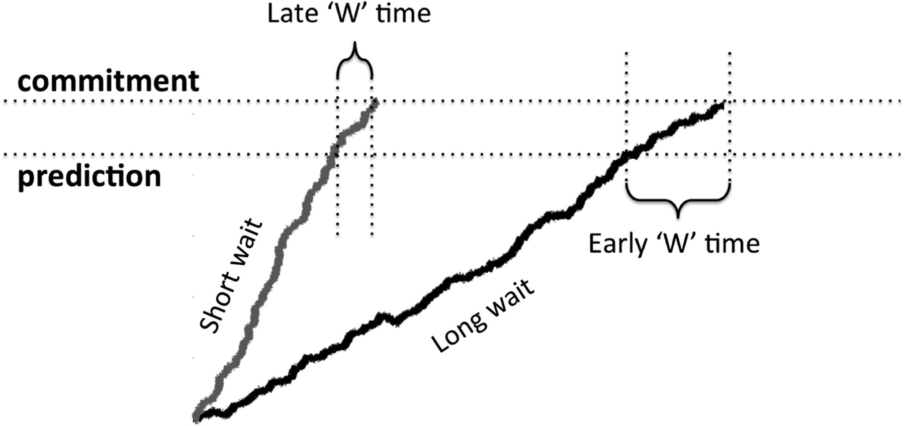
- Figure 7.
Predicting ‘W’ time as a function of waiting time. Schematic showing how ‘W’ time is predicted to vary as a function of waiting time. On trials with a short waiting time, the slope of the decision variable is steeper (gray line) than on trials with a long waiting time (black line). A steeper slope means that the interval between the crossing of the two thresholds will be shorter, so ‘W’ time will be closer in time to the onset of movement (smaller in absolute value). For trials with a more gradual slope of the decision variable (black line) the reverse is true, ‘W’ time will be further back in time from the onset of movement and larger in absolute value.
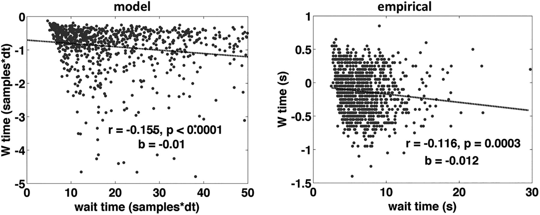
- Figure 8.
‘W’ time as a function of waiting time aggregate. Correlation between waiting time and ‘W’ time for simulated data from the model (left) and for the empirical data from all subjects (right; each dot is one trial from one subject). Although there is noise in the model, the model data are bounded by zero at the top, because there is no noise in the estimation of ‘W’ time, it is strictly earlier than movement time and is “reported” exactly as is. In reality there is a lot of variance across trials and across subjects in the reporting of ‘W’ time, and this is evident in the panel on the right. Combining the data from all subjects can be problematic, because differences between subjects and differences within subject are confounded, so in Figure 9, I present the correlations separately for each subject.
- Figure 9.
‘W’ time as a function of waiting time per subject. Correlation between waiting time and ‘W’ time for the empirical data grouped by subject. The horizontal axis is the waiting time (from 0 to 20 s) and the vertical axis is ‘W’ time in seconds with respect to movement onset. Data are shown in red if the correlation is individually significant at p < 0.05. When the r values for all subjects are submitted to a Wilcoxon signed rank test the effect is significant at p < 0.001. Also, the probability of 13 subjects (out of 14) individually exhibiting a negative correlation is 0.0009 (binomial test).


Extended Data
Extended Data 1
Download Extended Data, ZIP file.
In this issue


