

Abstract
Understanding how sensory systems process information depends crucially on identifying which features of the stimulus drive the response of sensory neurons, and which ones leave their response invariant. This task is made difficult by the many nonlinearities that shape sensory processing. Here, we present a novel perturbative approach to understand information processing by sensory neurons, where we linearize their collective response locally in stimulus space. We added small perturbations to reference stimuli and tested if they triggered visible changes in the responses, adapting their amplitude according to the previous responses with closed-loop experiments. We developed a local linear model that accurately predicts the sensitivity of the neural responses to these perturbations. Applying this approach to the rat retina, we estimated the optimal performance of a neural decoder and showed that the nonlinear sensitivity of the retina is consistent with an efficient encoding of stimulus information. Our approach can be used to characterize experimentally the sensitivity of neural systems to external stimuli locally, quantify experimentally the capacity of neural networks to encode sensory information, and relate their activity to behavior.
Significance Statement
Understanding how sensory systems process information is an open challenge mostly because these systems have many unknown nonlinearities. A general approach to studying nonlinear systems is to expand their response perturbatively. Here, we apply such a method experimentally to understand how the retina processes visual stimuli. Starting from a reference stimulus, we tested whether small perturbations to that reference (chosen iteratively using closed-loop experiments) triggered visible changes in the retinal responses. We then inferred a local linear model to predict the sensitivity of the retina to these perturbations, and showed that this sensitivity supported an efficient encoding of the stimulus. Our approach is general and could be used in many sensory systems to characterize and understand their local sensitivity to stimuli.
Introduction
An important issue in neuroscience is to understand how sensory systems use their neural resources to represent information. A crucial step toward understanding the sensory processing performed by a given brain area is to characterize its sensitivity (Benichoux et al., 2017), by determining which features of the sensory input are coded in the activity of these sensory neurons, and which features are discarded. If a sensory area extracts a given feature from the sensory scene, any change along that dimension will trigger a noticeable change in the activity of the sensory system. Conversely, if the information about a given feature is discarded by this area, the activity of the area should be left invariant by a change along that feature dimension. To understand which information is extracted by a sensory network, we must determine which changes in the stimulus evoke a significant change in the neural response, and which ones leave the response invariant.
This task is made difficult by the fact that sensory structures process stimuli in a highly nonlinear fashion. At the cortical level, many studies have shown that the response of sensory neurons is shaped by multiple nonlinearities (Machens et al., 2004; Carandini et al., 2005). Models based on the linear receptive field are not able to predict the responses of neurons to complex, natural scenes. This is even true in the retina. While spatially uniform or coarse grained stimuli produce responses that can be predicted by quasi-linear models (Berry and Meister, 1998; Keat et al., 2001; Pillow et al., 2008), stimuli closer to natural scenes (Heitman et al., 2016) or with rich temporal dynamics (Berry et al., 1999; Olveczky et al., 2003) are harder to characterize, as they trigger nonlinear responses in the retinal output. These unknown nonlinearities challenge our ability to model stimulus processing and limit our understanding of how neural networks process information.
Here, we present a novel approach to measure experimentally the local sensitivity of a nonlinear network. Because any nonlinear function can be linearized around a given point, we hypothesized that, even in a sensory network with nonlinear responses, one can still define experimentally a local linear model that can well predict the network response to small perturbations around a given reference stimulus. This local model should only be valid around the reference stimulus, but it is sufficient to predict if small perturbations can be discriminated based on the network response.
This local model allows us to estimate the sensitivity of the recorded network to changes around one stimulus. This local measure characterizes the ability of the network to code different dimensions of the stimulus space, circumventing the impractical task of building a complete accurate nonlinear model of the stimulus-response relationship. Although this characterization is necessarily local and does not generalize to the entire stimulus space, one can hope to use it to reveal general principles that are robust to the chosen reference stimulus.
We applied this strategy to the retina. We recorded the activity of a large population of retinal ganglion cells stimulated by a randomly moving bar. We characterized the sensitivity of the retinal population to small stimulus changes, by testing perturbations around a reference stimulus. Because the stimulus space is of high dimension, we designed closed-loop experiments to probe efficiently a perturbation space with many different shapes and amplitudes. This allowed us to build a complete model of the population response in that region of the stimulus space, and to precisely quantify the sensitivity of the neural representation.
We then used this experimental estimation of the network sensitivity to tackle two long-standing issues in sensory neuroscience. First, when trying to decode neural activity to predict the stimulus presented, it is always difficult to know if the decoder is optimal or if it misses some of the available information. We show that our estimation of the network sensitivity gives an upper bound of the decoder performance that should be reachable by an optimal decoder. Second, the efficient coding hypothesis (Attneave, 1954; Barlow, 1961) postulates that neural encoding of stimuli has adapted to represent natural occurring sensory scenes optimally in the presence of limited resources. Testing this hypothesis for sensory structures that perform nonlinear computations on high dimensional stimuli is still an open challenge. Here, we found that the network sensitivity with respect to stimulus perturbations exhibits a peak as a function of the temporal frequency of the perturbation, in agreement with prediction from efficient coding theory. Our method paves the way toward testing efficient coding theory in nonlinear networks.
Materials and Methods
Extracellular recording
Experiments were performed on the adult Long Evans rat of either sex, in accordance with institutional animal care standards. The retina was extracted from the euthanized animal and maintained in an oxygenated Ames’ medium (Sigma-Aldrich). The retina was recorded extracellularly on the ganglion cell side with an array of 252 electrodes spaced by 60 µm (Multichannel Systems), as previously described (Marre et al., 2012). Single cells were isolated offline using SpyKING CIRCUS a custom spike sorting algorithm (Yger et al., 2016). We then selected 60 cells that were well separated (no violations of refractory period, i.e., no spikes separated by <2 ms), had enough spikes (firing rate larger than 0.5 Hz), had a stable firing rate during the whole experiment, and responded consistently to repetitions of a reference stimulus (see Materials and Methods/Stimulus).
Stimulus
The stimulus was a movie of a white bar on a dark background projected at a refresh rate of 50 Hz with a digital micromirror device. The bar had intensity 7.6 × 10¹¹ photons/cm– 2/s– 1, and 115-µm width. The bar was horizontal and moved vertically. The bar trajectory consisted in 17034 snippets of 0.9 s consisting in two reference trajectories repeated 391 times each, perturbations of these reference trajectories and 6431 random trajectories. Continuity between snippets was ensured by constraining all snippets to start and end in the middle of the screen with velocity 0. Random trajectories followed the statistics of an overdamped stochastic oscillator (Deny et al., 2017). We used a Metropolis-Hastings algorithm to generate random trajectories satisfying the boundary conditions. The two reference trajectories were drawn from that ensemble.
Perturbations
Stimulus perturbations were small changes in the middle portion of the reference trajectory, between 280 and 600 ms. A perturbation is denoted by its discretized time series with time step δt = 20 ms,  , with L = 16, over the 320 ms of the perturbation (bold symbols represent vectors and matrices throughout). Perturbations can be decomposed as
  , where
  is the amplitude, and
  the shape. Perturbations shapes were chosen to have zero value and zero derivative at their boundaries (Fig. 1).

Perturbations shapes. We used the same 16 perturbation shapes for the two reference stimuli. The first 12 perturbation shapes were combinations of two Fourier components, and the last four ones were random combinations of them:  and
and  , with T the duration of the perturbation and t = 0 the beginning of the perturbation. The first perturbations j = 1…7 were
  . For j = 8,…,10, they were the opposite of the three first ones:
  . For j = 11, 12 we used
  . Perturbations 13 and 14 were random combinations of perturbations 1, 2, 3, 11, and 12, constrained to be orthogonal. Perturbations 15 and 16 were random combinations of fj for j ∈ [1,8] and gk for k ∈ [1,7], allowing higher frequencies than perturbation directions 13 and 14. Perturbation direction 15 and 16 were also constrained to be orthogonal. The largest amplitude for each perturbation we presented was 115 µm. An exception was made for perturbations 15 and 16 applied to the second reference trajectory, as for this amplitude they had a discrimination probability below 70%. They were thus increased by a factor 1.5. The largest amplitude for each perturbation was repeated at least 93 times, with the exception of perturbation 15 (32 times) and 16 (40 times) on the second reference trajectory.
Closed-loop experiments
We aimed to characterize the population discrimination capacity of small perturbations to the reference stimulus. For each perturbation shape (Fig. 1), we searched for the smallest amplitude that will still evoke a detectable change in the retinal response, as we explain below. To do this automatically on the many tested perturbation shapes, we implemented closed-loop experiments (Fig. 3A). At each iteration, the retina was stimulated with a perturbed stimulus and the population response was recorded and used to select the next stimulation in real time.
Online spike detection
During the experiment we detected spikes in real time on each electrode independently. Each electrode signal was high-pass filtered using a Butterworth filter with a 200-Hz frequency cutoff. A spike was detected if the electrode potential U was lower than a threshold of five times the median absolute deviation of the voltage (Yger et al., 2016).
Online adaptation of perturbation amplitude
To identify the range of perturbations that were neither too easy nor too hard to discriminate, we adapted perturbation amplitudes so that the linear discrimination probability (see below) converged to target value D* = 85%. For each shape, perturbation amplitudes were adapted using the Accelerated Stochastic Approximation (Kesten, 1958). If an amplitude An triggered a response with discrimination probability Dn, then at the next step the perturbation was presented at amplitude An+1 with (1)where C = 0.74 is a scaling coefficient that controls the size of steps, and rn is the number of reversal steps in the experiment, i.e., the number of times when a discrimination Dn larger than D
* was followed by Dn+1 smaller than D
*, and vice versa. to explore the responses to different ranges of amplitudes even in the case where the algorithm converged too fast, we also presented amplitudes regularly spaced on a log-scale. We presented the largest amplitude Amax (Fig. 1, value), and scaled it down by multiples of 1.4,
(1)where C = 0.74 is a scaling coefficient that controls the size of steps, and rn is the number of reversal steps in the experiment, i.e., the number of times when a discrimination Dn larger than D
* was followed by Dn+1 smaller than D
*, and vice versa. to explore the responses to different ranges of amplitudes even in the case where the algorithm converged too fast, we also presented amplitudes regularly spaced on a log-scale. We presented the largest amplitude Amax (Fig. 1, value), and scaled it down by multiples of 1.4,  with k = 1,…,7.
Online and offline linear discrimination
We applied linear discrimination theory to estimate if perturbed and reference stimuli can be discriminated from the population response they trigger. We applied it twice: online, on the electrode signals to adapt the perturbation amplitude, and offline, on the sorted spikes to estimate the response discrimination capacity. The response  over time of either the N = 256 electrodes, or the N = 60 cells (the same notation N and R are used for electrode number and response and cell number and response for mathematical convenience), was binarized into B time bins of size δ = 20 ms: Rib = 1 if cell i spiked at least once during the bth time bin, and 0 otherwise. R is thus a vector of size N × B, labeled by a joint index ib. The response is considered from the start of the perturbation until 280 ms after its end, so that B = 30.
To apply linear discrimination on  , the response to the perturbation S, we record multiple responses
  to the reference, and multiple responses
  to a large perturbation
  , with the same stimulus shape as S but at the maximum amplitude that was played during the course of the experiment (typically 110 μm; Fig. 1). Our goal is to estimate how close
  is to the “typical”
  compared to the typical
  . To this aim, we compute the mean response to the reference and to the large perturbation,
  and
and  , and use their difference as a linear classifier. Specifically, we project
  onto the difference between these two mean responses. For a generic response
  (either
  or
or  ), the projection x (respectively,
  or
or  ) reads:
 (2)where x is a scalar and
  is the linear discrimination axis. The computation of x is a projection in our joint index notation, but it can be decomposed in a summation over cells i and consecutive time-bins b of the response:
  . On average, we expect
  . To quantify the discrimination capacity, we compute the probability that
  , following the classical approach for linear classifiers.
To avoid overfitting, when projecting a response to the reference trajectory,  , onto
  , we first re-compute
  by leaving out the response of interest. If we did not do this, the discriminability of responses would be overestimated.
In Discussion, Mathematical derivations, we discuss the case of a system with response changes that are linear in the perturbation, or equivalently when the perturbation is small enough so that a linear first order approximation is valid.
Offline discrimination and sensitivity
To measure the discrimination probability as a function of the perturbation amplitude, we consider the difference of the projections,  . The response to the stimulation
  is noisy, making x and xref the sum of many random variables (corresponding to each neuron and time bin combinations), and we can apply the central limit theorem to approximate their distributions as Gaussian (Fig. 3B, right side), for a given perturbation at a given amplitude. For small perturbations, the mean of Δx grows linearly with the perturbation amplitude A, μ = α × A, and the variances of
  and
and  are equal at first order,
  , so that the variance of Δx,
  is independent of A. Then the probability of discrimination is given by the error function:
 (3)
where
(3)
where  is the standard sensitivity index (Macmillan and Creelman, 2004), and c = α∕σ is defined as the sensitivity coefficient, which depends on the perturbation shape Q. This coefficient determines the amplitude A = c
– 1 at which discrimination probability is equal to
is the standard sensitivity index (Macmillan and Creelman, 2004), and c = α∕σ is defined as the sensitivity coefficient, which depends on the perturbation shape Q. This coefficient determines the amplitude A = c
– 1 at which discrimination probability is equal to  .
.
Optimal sensitivity and Fisher information
We then aimed to find the discrimination probability for any perturbation. Given the distributions of responses to the reference stimulus,  , and to a perturbation,
  , optimal discrimination can be achieved by studying the sign of the response-specific log-ratio
  . Note that in the log-ratio, R represents a stochastic response and not the independent variable of a probability density. Because it depends on the response R, this log ratio is both stimulus dependent and stochastic. Let us define
  to be the random variable taking value
  on presentation of the reference stimulus, i.e., when R is a (stochastic) response to the stimulus, and
  the random variable taking value
  when R is a response to the presentation of S. According to the definition given earlier, the probability of successful discrimination is the probability that the log-ratio calculated from a random response to the perturbed stimulus is larger than the log-ratio calculated from a random response to the reference,
  . Using the central limit theorem, we assume again that
  and
and  are Gaussian. We can calculate their mean and variance at small S (see Discussion, Mathematical derivations):
  and
and  , where
 (4)is the Fisher information matrix calculated at the reference stimulus. Following standard discrimination theory (Macmillan and Creelman, 2004; for a derivation in a similar context, see Seung and Sompolinsky, 1993), the discrimination probability is (see Discussion, Mathematical derivations):
  , with
 (5)
(5)
This result generalizes to an arbitrary stimulus dimension the result of Seung and Sompolinsky (1993).
Local model
Because sampling the full response probability distribution  would require estimating 2
N
×
B numbers (one for each possible response R) for each perturbation S, estimating the Fisher Information Matrix directly is impractical, and requires building a model that can predict how the retina responds to small perturbations of the reference stimulus. We used the data from these closed loop experiments for this purpose. The model, schematized in Figure 4A, assumes that a linear correction can account for the response change driven by small perturbations. We introduce the local model as a linear expansion of the logarithm of response distribution as a function of both stimulus and response:
would require estimating 2
N
×
B numbers (one for each possible response R) for each perturbation S, estimating the Fisher Information Matrix directly is impractical, and requires building a model that can predict how the retina responds to small perturbations of the reference stimulus. We used the data from these closed loop experiments for this purpose. The model, schematized in Figure 4A, assumes that a linear correction can account for the response change driven by small perturbations. We introduce the local model as a linear expansion of the logarithm of response distribution as a function of both stimulus and response:
 (6)
where in the integral form, {ti} denotes the set of spiking times of neuron i, and Fi is a stimulus filter depending on both the stimulus time and spiking time (no time-translation invariance). The second line is the discretized version adapted to our binary convention for describing spiking activity binned into bins indexed by b. The matrix
(6)
where in the integral form, {ti} denotes the set of spiking times of neuron i, and Fi is a stimulus filter depending on both the stimulus time and spiking time (no time-translation invariance). The second line is the discretized version adapted to our binary convention for describing spiking activity binned into bins indexed by b. The matrix  is the discretized version of
  and contains the linear filters with which the change in the response is calculated from the linear projection of the past stimulus. For ease of notation, hereafter we use matrix multiplications rather than explicit sums over ib and t.
The distribution of responses to the reference trajectory is assumed to be conditionally independent: (7)
(7)
Since the variables Rib are binary, their mean values ⟨Rib⟩ on presentation of the reference completely specify  :
:  . They are directly evaluated from the responses to repetitions of the reference stimulus, with a small pseudo-count to avoid zero values.
Evaluating the Fisher information matrix (Eq. 4), within the local model (Eq. 6), gives: (8)where
  is the covariance matrix of R, which within the model is diagonal because of the assumption of conditional independence.
Inference of the local model
To infer the filters Fib,t, we only include perturbations that are small enough to remain within the linear approximation. We first separated the dataset into a training (285 × 16 perturbations) and testing (20 × 16 perturbations) sets. We then defined, for each perturbation shape, a maximum perturbation amplitude above which the linear approximation was no longer considered valid. We selected this threshold by optimizing the model’s ability to predict the changes in firing rates in the testing set. Model learning was performed for each cell independently by maximum likelihood with an L2 smoothness regularization on the shape of the filters, using a pseudo-Newton algorithm. The amplitude threshold obtained from the optimization varied widely across perturbation shapes. The number of perturbations for each shape used in the inference ranged from 20 (7% of the total) to 260 (91% of the total). Overall only 32% of the perturbations were kept (as we excluded repetitions of perturbations with largest amplitude used for calibration). Overfitting was limited: when tested on perturbations of similar amplitudes, the prediction performance on the testing set was never lower than 15% of the performance on the training set.
Linear decoder
We built a linear decoder of the bar trajectory from the population response. The model takes as input the population response R to the trajectory X(t) and provides a prediction  of the bar position in time:
 (9)where the filters K have a time integration windows of 15 × 20 ms = 300 ms, as in the local model.
We inferred the linear decoder filters by minimizing the mean square error (Warland et al., 1997),  , in the reconstruction of 4000 random trajectories governed by the dynamics of an overdamped oscillator with noise (see Materials and Methods/Stimulus). The linear decoder is then applied to the perturbed trajectories, X(t) = X0(t) + S(t), where X0(t) denotes the reference trajectory. The linear decoder does not use prior information about the local structure of the experiment, namely about the fact that the stimulus to decode consists of perturbations around a reference simulation. However, it implicitly uses prior information about the statistics of the overdamped oscillator, as it was trained on bar trajectories with those statistics. Tested on a sequence of ∼400 repetitions of one of the two reference trajectories, where the first 300 ms of each have been cut out, we obtain a correlation coefficient of 0.87 between the stimulus and its reconstruction.
Local model Bayesian decoder
To construct a decoder based on the local model, we use Bayes’ rule to infer the presented stimulus given the response: (10)where
  is given by the local model (Eq. 6),
  is the prior distribution over the stimulus, and
  is the prior distribution over the stimulus, and
  is a normalization factor that does not depend on the stimulus.
  is taken to be the distribution of trajectories from an overdamped stochastic oscillator with the same parameters as in the experiment (Deny et al., 2017), to allow for a fair comparison with the linear decoder, which was trained with those statistics. The stimulus is inferred by maximizing the posterior
  numerically, using a pseudo-Newton iterative algorithm.
Local signal to noise ratio in decoding
To quantify local decoder performance as a function of the stimulus frequency, we estimated a local signal-to-noise ratio (LSNR) of the decoding signal, LSNR(S), which is a function of the reference stimulus. Here, we cannot compute SNR as a ratio between total signal power and noise power, because this would require to integrate over the entire stimulus space, while our approach only provides a model around the neighborhood of the reference stimulus.
To obtain a meaningful comparison between the linear and local decoders, we expand them at first order in the stimulus perturbation and compute the SNR of these “linearized” decoders. For any decoder and for stimuli nearby a reference stimulation, the inferred value of the stimulus,  , can be written as
  , where X is the real bar trajectory, and
  has a random component (due to the random nature of the response on which the reconstruction relies). Linearizing
  for
for  ,
,
 (11)where T is a transfer matrix which differs from the identity matrix when decoding is imperfect, and
  a Gaussian noise of covariance
  . Thus, the reconstructed perturbation
  can be written as:
 (12)
where
(12)
where  is a systematic bias. We inferred the values of b and
  from the ∼400 reconstructions of the reference stimulation using either of the two decoders, and the values of T from the reconstructions of the perturbed trajectories. The inference is done by an iterative algorithm similar to that used for the inference of the filters F of the local model. We define the LSNR in decoding the perturbation S as:
 (13)where here
  means average with respect to the noise
  . In this formula, the signal is defined as the average predicted perturbation
  , from which the systematic bias b is subtracted, yielding
  . The noise is simply ϵ. Note that here the LSNR is defined for a given perturbation S. It is the ratio of the squared signal to the noise variance (summed over the eigendirections of the noise correlator, since we are dealing with a multidimensional signal). This LSNR gives a measure of decoding performance, through the amplitude of the decoded signal relative to the noise. To study how this performance depends on the frequency ν of the input signal, in Figure 6C, we apply Equation 13 with
  , where A is the amplitude of the perturbation (Fig. 5A), and b is a time-bin counter. Note that this frequency-dependent LSNR should not be intepreted as a ratio of signal and noise power spectra, but rather as the dependence of decoding performance on the frequency of the perturbation. It is used rather than the traditional SNR because we are dealing with signals with no time-translation invariance (i.e.,
  is not just a function of
  , and neither is
  ). However, our LNSR reduces to the traditional frequency-dependent SNR in the special case of time-translation invariance, i.e., when the decoder is convolutional, and its noise stationary (see Discussion, Mathematical derivations)
Fisher information estimation of sensitivity coefficients
In Figures 5A,B, 7C,D, we show the Fisher estimations of sensitivity coefficients  for perturbations of different shapes Q, either those used during the experiment (Fig. 1), or oscillating ones,
  . to compute these sensitivity coefficients, we use Equation 14 to compute the sensitivity index
  and then we divide it by the perturbation amplitude, yielding
  .
.
Results
Measuring sensitivity using closed-loop experiments
We recorded from a population of 60 ganglion cells in the rat retina using a 252-electrode array while presenting a randomly moving bar (Fig. 2A; Materials and Methods). Tracking the position of moving objects is major task that the visual system needs to solve. The performance in this task is constrained by the ability to discriminate different trajectories from the retinal activity. Our aim was to measure how this recorded retinal population responded to different small perturbations around a pre-defined stimulus. We measured the response to many repetitions of a short (0.9 s) reference stimulus, as well as many small perturbations around it. The reference stimulus was the random trajectory of a white bar on a dark background undergoing Brownian motion with a restoring force (see Materials and Methods). Perturbations were small changes affecting that reference trajectory in its middle portion, between 280 and 600 ms. The population response was defined as sequences of spikes and silences in 20-ms time bins for each neuron, independently of the number of spikes (see Materials and Methods).

Sensitivity of a neural population to visual stimuli. A, The retina is stimulated with repetitions of a reference stimulus (here the trajectory of a bar, in blue), and with perturbations of this reference stimulus of different shapes and amplitudes. Purple and red trajectories are perturbations with the same shape, of small and large amplitude. B, Mean response of three example cells to the reference stimulus (left column and light blue in middle and right columns) and to perturbations of small and large amplitudes (middle and right columns).
To assess the sensitivity of the retinal network, we asked how well different perturbations could be discriminated from the reference stimulus based on the population response. We expect the ability to discriminate perturbations to depend on two factors. First, the direction of the perturbation in the stimulus space, called perturbation shape. If we change the reference stimulus by moving along a dimension that is not taken into account by the recorded neurons, we should not see any change in the response. Conversely, if we choose to change the stimulus along a dimension that neurons “care about,” we should quickly see a change in the response. The second factor is the amplitude of the perturbation: responses to small perturbations should be hardly distinguishable, while large perturbations should elicit easily detectable changes (Fig. 2B). To assess the sensitivity to perturbations of the reference stimulus we need to explore many possible directions that these perturbations can take, and for each direction, we need to find a range of amplitudes that is as small as possible but will still evoke a detectable change in the retinal response. In other words, we need to find the range of amplitudes for which discrimination is hard but not impossible. This requires looking for the adequate range of perturbation amplitudes “online,” during the time course of the experiment.
To automatically adapt the amplitude of perturbations to the sensitivity of responses for each of the 16 perturbation shapes and for each reference stimulus, we implemented closed-loop experiments (Fig. 3A). At each step, the retina was stimulated with a perturbed stimulus and the population response was recorded. Spikes were detected in real time for each electrode independently by threshold crossing (see Materials and Methods). This coarse characterization of the response is no substitute for spike sorting, but it is fast enough to be implemented in real time between two stimulus presentations, and sufficient to detect changes in the response. This method was used to adaptively select the range of perturbations in real time during the experiment, and to do it for each direction of the stimulus space independently. Proper spike sorting was performed after the experiment using the procedure described in Marre et al., 2012 and Yger et al., (2016) and used for all subsequent analyses.

Closed-loop experiments to probe the range of stimulus sensitivity. A, Experimental setup: we stimulated a rat retina with a moving bar. Retinal ganglion cell (RGC) population responses were recorded extracellularly with a multielectrode array. Electrode signals were high-pass filtered and spikes were detected by threshold crossing. We computed the discrimination probability of the population response and adapted the amplitude of the next perturbation. B, left, The neural responses of 60 sorted RGCs are projected along the axis going through the mean response to reference stimulus and the mean response to a large perturbation. Small dots are individual responses, large dots are means. Middle, Mean and standard deviation (in gray) of response projections for different amplitudes of an example perturbation shape. Right, Distributions of the projected responses to the reference (blue), and to small (purple) and large (red) perturbations. Discrimination is high when the distribution of the perturbation is well separated from the distribution of the reference. C, Discrimination probability as a function of amplitude A. The discrimination increases as an error function,  , with
  (gray line: fit). Ticks on the x-axis show the amplitudes that have been tested during the closed-loop experiment.
To test whether a perturbation was detectable from the retinal response, we considered the population response, summarized by a binary vector containing the spiking status of each recorded neuron in each time bin, and projected it onto an axis to obtain a single scalar number. The projection axis was chosen to be the difference between the mean response to a large-amplitude perturbation and the mean response to the reference (Fig. 3B). On average, the projected response to a perturbation is larger than the projected response to the reference. However, this may not hold for individual responses, which are noisy and broadly distributed around their mean (for example distributions, see Fig. 3B, right). We define the discrimination probability as the probability that the projected response to the perturbation is in fact larger than to the reference. Its value is 100% if the responses to the reference and perturbation are perfectly separable, and 50% if their distributions are identical, in which case the classifier does no better than chance. This discrimination probability is equal to the “area under the curve of the receiver-operating characteristics,” which is widely used for measuring the performance of binary discrimination tasks.
During our closed-loop experiment, our purpose was to find the perturbation amplitude with a discrimination probability of 85%. To this end, we computed the discrimination probability online as described above, and then chose the next perturbation amplitude to be displayed using the “accelerated stochastic approximation” method (Kesten, 1958; Faes et al., 2007): when discrimination was above 85%, the amplitude was decreased, otherwise, it was increased (see Materials and Methods).
Figure 3C shows the discrimination probability as a function of the perturbation amplitude for an example perturbation shape. Discrimination grows linearly with small perturbations, and then saturates to 100% for large ones. This behavior is well approximated by an error function (gray line) parametrized by a single coefficient, which we call sensitivity coefficient and denote by c. This coefficient measures how fast the discrimination probability increases with perturbation amplitude: the higher the sensitivity coefficient, the easier it is to discriminate responses to small perturbations. It can be interpreted as the inverse of the amplitude at which discrimination reaches 76%, and is related to the classical sensitivity index  (Macmillan and Creelman, 2004), through
  , where A denotes the perturbation amplitude (see Materials and Methods).
All 16 different perturbation shapes were displayed, corresponding to 16 different directions in the stimulus space, and the optimal amplitude was searched for each of them independently. We found a mean sensitivity coefficient of c = 0.0516 μm– 1. However, there were large differences across the different perturbation shapes, with a minimum of c = 0.028 μm– 1 and a maximum of c = 0.065 μm– 1.
Sensitivity and Fisher information
So far, our results have allowed us to estimate the sensitivity of the retina in specific directions of the perturbation space. Can we generalize from these measurements and predict the sensitivity in any direction? The stimulus is the trajectory of a bar and is high dimensional. Under the assumptions of the central limit theorem, we show that the sensitivity can be expressed in matrix form as (see Materials and Methods):
 (14)where I is the Fisher information matrix, of the same dimension as the stimulus, and S the perturbation represented as a column vector. This result generalizes that of Seung and Sompolinsky (1993), initially derived for one-dimensional stimuli, to arbitrary dimensions. Thus, the Fisher information is sufficient to predict the code’s sensitivity to any perturbation.
Despite the generality of Equation 14, it should be noted that estimating the Fisher information matrix for a highly dimensional stimulus ensemble requires a model of the population response. As already discussed in the introduction, the nonlinearities of the retinal code make the construction of a generic model of responses to arbitrary stimuli a very arduous task, and is still an open problem. However, the Fisher information matrix need only be evaluated locally, around the response to the reference stimulus, and to do so building a local response model is sufficient.
Local model for predicting sensitivity
We introduce a local model to describe the stochastic population response to small perturbations of the reference stimulus. This model will then be used to estimate the Fisher information matrix, and from it the retina’s sensitivity to any perturbation, using Equation 14.
The model, schematized in Figure 4A, assumes that perturbations are small enough that the response can be linearized around the reference stimulus. First, the response to the reference is described by conditionally independent neurons firing with time-dependent rates estimated from the peristimulus time histograms (PSTHs). Second, the response to perturbations is modeled as follows: for each neuron and for each 20-ms time bin of the considered response, we use a linear projection of the perturbation trajectory onto a temporal filter to modify the spike rates relative to the reference. These temporal filters were inferred from the responses to all the presented perturbations, varying both in shape and amplitude (but small enough to remain within the linear approximation). Details of the model and its inference are given in Materials and Methods.

Local model for responses to perturbations. A, The firing rates in response to a perturbation of a reference stimulus are modulated by filters applied to the perturbation. There is a different filter for each cell and each time bin. Because the model is conditionally independent across neurons we show the schema for one example neuron only. B, Raster plot of the responses of an example cell to the reference (blue) and perturbed (red) stimuli for several repetitions. C, PSTH of the same cell in response to the same reference (blue) and perturbation (red). Prediction of the local model for the perturbation is shown in green. D, Performance of the local model at predicting the change in PSTH induced by a perturbation, as measured by Pearson correlation coefficient between data and model, averaged over cells (green). The data PSTH were calculated by grouping perturbations of the same shape and of increasing amplitudes by groups of 20 and computing the mean firing rate at each time over the 20 perturbations of each group. The model PSTH was calculated by mimicking the same procedure. To control for noise from limited sampling, the same performance was calculated from synthetic data of the same size, where the model is known to be exact (black).
We checked the validity of the local model by testing its ability to predict the PSTH of cells in response to perturbations (Fig. 4B). To assess model performance, we computed the difference of PSTH between perturbation and reference, and compared it to the model prediction. Figure 4D shows the correlation coefficient of this PSTH difference between model and data, averaged over all recorded cells for one perturbation shape. To obtain an upper bound on the attainable performance given the limited amount of data, we computed the same quantity for responses generated by the model (black line). Model performance saturates that bound for amplitudes up to 60 μm, indicating that the local model can accurately predict the statistics of responses to perturbations within that range. For larger amplitudes, the linear approximation breaks down, and the local model fails to accurately predict the response. This failure for large amplitudes is expected if the retinal population responds nonlinearly to the stimulus. We observed the same behavior for all the perturbation shapes that we tested. We have therefore obtained a local model that can predict the response to small enough perturbations in many directions.
To further validate the local model, we combine it with Equation 14 to predict the sensitivity c of the network to various perturbations of the bar trajectory, as measured directly by linear discrimination (Fig. 3). The Fisher matrix takes a simple form in the local model:  , where F is the matrix containing the model’s temporal filters (stacked as row vectors), and
  is the covariance matrix of the entire response to the reference stimulus across neurons and time. We can then use the Fisher matrix to predict the sensitivity coefficient using Equation 14, and compare it to the same sensitivity coefficient previously estimated using linear discrimination. Figure 5A shows that these two quantities are strongly correlated (Pearson correlation: 0.82, p = 10–8), although the Fisher prediction is always larger. This difference could be due to two reasons: limited sampling of the responses, or nonoptimality of the projection axis used for linear discrimination. To evaluate the effect of finite sampling, we repeated the analysis on a synthetic dataset generated using the local model, with the same stimulation protocol as in the actual experiment. The difference in the synthetic data (Fig. 5B) and experiment (Fig. 5A) were consistent, suggesting that finite sampling is indeed the main source of discrepancy. We confirmed this result by checking that using the optimal discrimination axis (see Discussion, Mathematical derivations) did not improve performance (data not shown).
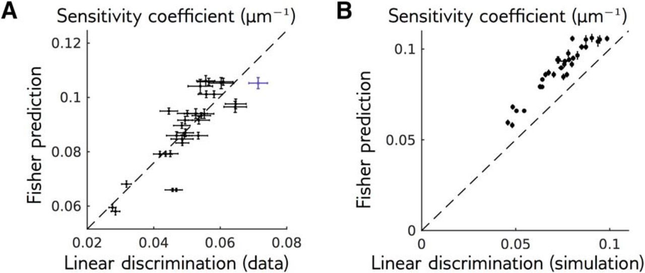
The Fisher information predicts the experimentally measured sensitivity. A, Sensitivity coefficients c for the two reference stimuli and 16 perturbation shapes, measured empirically and predicted by the Fisher information (Eq. 14) and the local model. The purple point corresponds to the perturbation shown in Figure 2. Dashed line stands for best linear fit. B, Same as A, but for responses simulated with the local model, with the same amount of data as in experiments. The discriminability of perturbations was measured in the same way than for recorded responses. Dots and error bars stand for mean and SEM over 10 simulations. Dashed line stands for identity.
Summarizing, our estimation of the local model and of the Fisher information matrix can predict the sensitivity of the retinal response to perturbations in many directions of the stimulus space. We now use this estimation of the sensitivity of the retinal response to tackle two important issues in neural coding: the performance of linear decoding and efficient information transmission.
Linear decoding is not optimal
When trying to decode the position of random bar trajectories over time using the retinal activity, we found that a linear decoder (see Materials and Methods) could reach a satisfying performance, confirming previous results (Warland et al., 1997 and Marre et al., 2015). Several works have shown that it was challenging to outperform linear decoding on this task in the retina (Warland et al., 1997 and Marre et al., 2015). From this result, we can wonder whether the linear decoder is optimal, i.e., makes use of all the information present in the retinal activity, or whether this decoder is suboptimal and could be outperformed by a nonlinear decoder. To answer this question, we need to determine an upper bound on the decoding performance reachable by any decoding method. For an encoding model, the lack of reliability of the response sets an upper bound on the encoding model performance, but finding a similar upper bound for decoding is an open challenge. Here, we show that our local model can define such an upper bound.
The local model is an encoding model: it predicts the probability of responses given a stimulus. Yet it can be used to create a “Bayesian decoder” using Bayesian inversion (see Materials and Methods): given a response, what is the most likely stimulus that generated this response under the model? Since the local model predicts the retinal response accurately, doing Bayesian inversion of this model should be the best decoding strategy, meaning that other decoders should perform equally or worse. When decoding the bar trajectory, we found that the Bayesian decoder was more precise than the linear decoder, as measured by the variance of the reconstructed stimulus (Fig. 6A). The Bayesian decoder had a smaller error than the linear decoder when decoding perturbations of small amplitudes (Fig. 6B). For larger amplitudes, where the local model is expected to break down, the performance of the Bayesian decoder decreased.
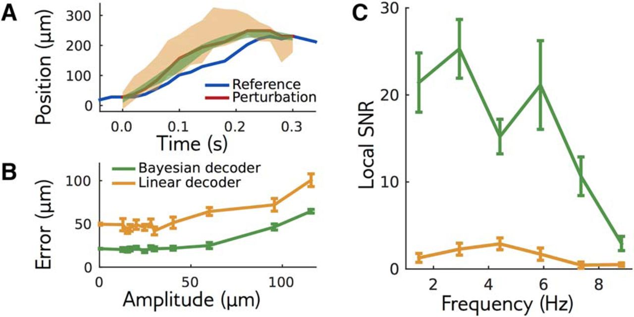
Bayesian decoding of the local model outperforms the linear decoder. A, Responses to a perturbation of the reference stimulus (reference in blue, perturbation in red) are decoded using the local model (green) or a linear decoder (orange). For each decoder, the area shows one standard deviation from the mean. B, Decoding error as a function of amplitude, for an example perturbation shape. C, LSNR for perturbations with different frequencies (differing from the standard SNR definition to deal with locality in stimulus space and in time; Materials And Methods/Local signal to noise ratio in decoding). The performance of both decoders decreases for high frequency stimuli.
To quantify decoding performance as a function of the stimulus temporal frequency, we estimated a “LSNR” of the decoding signal for small perturbations of various frequencies (see Materials and Methods). The definition of the LSNR differs from the usual frequency-dependent SNR, as it is defined to deal with signals that are local in stimulus space and in time, i.e., with no invariance to time translations. We verified however that the two are equivalent when time-translation invariance is satisfied (see Discussion, Mathematical derivations). The Bayesian decoder had a much higher LSNR than the linear decoder at all frequencies (Fig. 6C), even if both did fairly poorly at high frequencies. This shows that, despite its good performance, linear decoding misses some information about the stimulus present in the retinal activity. This result suggests that inverting the local model, although it does not provide an alternative decoder generalizable to all possible trajectories, sets a gold standard for decoding, and can be used to test whether other decoders miss a significant part of the information present in the neural activity. It also confirms that the local model is an accurate description of the retinal response to small enough perturbations around the reference stimulus.
Signature of efficient coding in the sensitivity
The structure of the Fisher information matrix shows that the retinal population is more sensitive to some directions of the stimulus space than others. Are these differences in the sensitivity optimal for efficient information transmission? We hypothesized that the retinal sensitivity has adapted to the statistics of the bar motion presented throughout the experiment to best transmit information about its position. Figure 7A represents the power spectrum of the bar motion, which is maximum at low frequencies, and quickly decays at large frequencies. We used our measure of the Fisher matrix to estimate the retinal sensitivity power as the sensitivity coefficient c to oscillatory perturbations as a function of temporal frequency (see Materials and Methods). Unlike the power spectrum, which depends monotonously on frequency, we found that the sensitivity is bell shaped, with a peak in frequency around 4Hz (Fig. 7C).
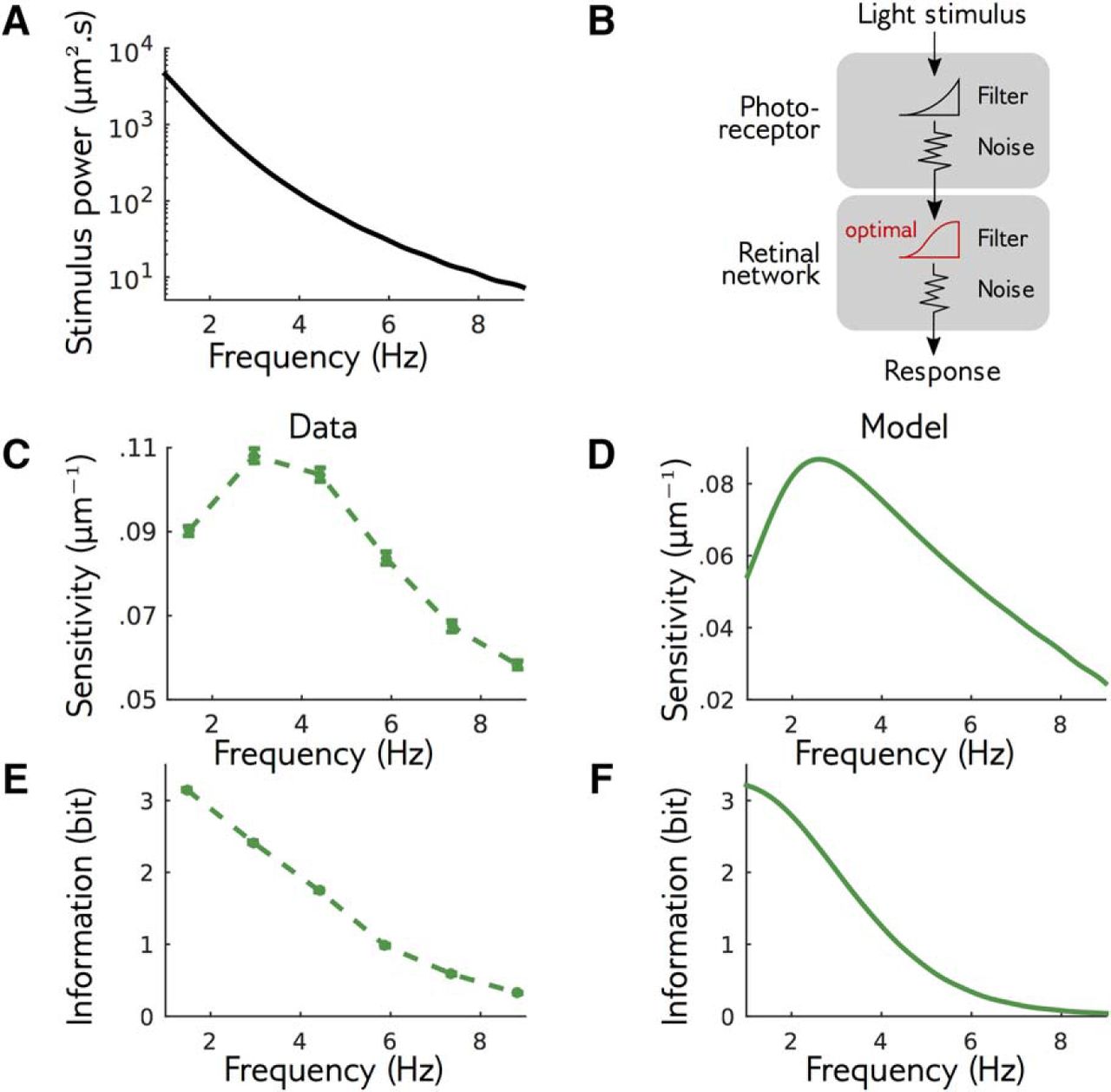
Signature of efficient coding in the sensitivity. A, Spectral density of the stimulus used in experiments, which is monotonically decreasing. B, Simple theory of retinal function: the stimulus is filtered by noisy photoreceptors, whose signal is then filtered by the noisy retinal network. The retinal network filter was optimized to maximize information transfer at constant output power. C, Sensitivity of the recorded retina to perturbations of different frequencies. Note the nonmonotonic behavior. D, Same as C, but for the theory of optimal processing. E, Information transmitted by the retina on the perturbations at different amplitudes. F, Same as E, but for the theory.
To interpret this peak in sensitivity, we studied a minimal theory of retinal function, similar to Van Hateren (1992), to test how maximizing information transmission would reflect on the sensitivity of the retinal response. In this theory, the stimulus is first passed through a low-pass filter, then corrupted by an input white noise. This first stage describes filtering due to the photoreceptors (Ruderman and Bialek, 1992). The photoreceptor output is then transformed by a transfer function and corrupted by a second external white noise, which mimics the subsequent stages of retinal processing leading to ganglion cell activity. Here the output is reduced to a single continuous signal (Fig. 7B; for details, see Discussion, Mathematical derivations). Note that this theory is linear: we are not describing the response of the retina to any stimulus, which would be highly nonlinear, but rather its linearized response to perturbations around a given stimulus, as in our experimental approach. To apply the efficient coding hypothesis, we assumed that the photoreceptor filter is fixed, and we maximized the transmitted information, measured by Shannon’s mutual information, over the transfer function (see Discussion, Mathematical derivations; Eq. 31). We constrained the variance of the output to be constant, corresponding to a metabolic constraint on the firing rate of ganglion cells. In this simple and classical setting, this optimal transfer function, and the corresponding sensitivity, can be calculated analytically. Although the power spectrum of the stimulus and photoreceptor output are monotonically decreasing, and the noise spectrum is flat, we found that the optimal sensitivity of the theory is bell shaped (Fig. 7E), in agreement with our experimental findings (Fig. 7C). Recall that in our reasoning, we assumed that the network optimizes information transmission for the statistics of the stimulus used in the experiment. Alternatively, it is possible that the retinal network optimizes information transmission of natural stimuli, which may have slightly different statistics. We also tested our model with natural temporal statistics (power spectrum ∼1∕ν 2 as a function of frequency ν; Dong and Atick, 1995) and found the same results (data not shown).
One can intuitively understand our result that a bell-shaped sensitivity is desirable from a coding perspective. On one hand, in the small frequency regime, sensitivity increases with frequency, i.e., decreases with stimulus power. This result is classic: when the input noise is small compared to stimulus, the best coding strategy for maximizing information is to whiten the input signal to obtain a flat output spectrum, which is obtained by having the squared sensitivity be inversely proportional to the stimulus power (Rieke et al., 1996; Wei and Stocker, 2016). On the other hand, at high frequencies, the input noise is too high (relative to the stimulus power) for the stimulus to be recovered. Allocating sensitivity and output power to those frequencies is therefore a waste of resources, as it is devoted to amplifying noise, and sensitivity should remain low to maximize information. A peak of sensitivity is thus found between the high SNR region, where stimulus dominates noise and whitening is the best strategy, and the low LSNR region, where information is lost into the noise and coding resources should be scarce. A result of this optimization is that the information transferred should monotonically decrease with frequency, just as the input power spectrum does (Fig. 7F). We tested if this prediction was verified in the data. We estimated similarly the information rate against frequency in our data, and found that it was also decreasing monotonically (Fig. 7D). The retinal response has therefore organized its sensitivity across frequencies in a manner that is consistent with an optimization of information transmission across the retinal network.
Discussion
We have developed an approach to characterize experimentally the sensitivity of a sensory network to changes in the stimulus. Our general purpose was to determine which dimensions of the stimulus space most affect the response of a population of neurons, and which ones leave it invariant, a key issue to characterize the selectivity of a neural network to sensory stimuli. We developed a local model to predict how recorded neurons responded to perturbations around a defined stimulus. With this local model we could estimate the sensitivity of the recorded network to changes of the stimulus along several dimensions. We then used this estimation of network sensitivity to show that it can help define an upper bound on the performance of decoders of neural activity. We also showed that the estimated sensitivity was in agreement with the prediction from efficient coding theory.
Our approach can be used to test how optimal different decoding methods are. In our case, we found that linear decoding, despite its very good performance, was far from the performance of the Bayesian inversion of our local model, and therefore far from optimal. This result implies that there should exist nonlinear decoding methods that outperform linear decoding (Botella-Soler et al., 2016). Testing the optimality of the decoding method is crucial for brain machine interfaces (Gilja et al., 2012): in this case, an optimal decoder is necessary to avoid missing a significant amount of information. Building our local model is a good strategy for benchmarking different decoding methods.
In the retina, efficient coding theory had led to key predictions about the shape of the receptive fields, explaining their spatial extent (Atick, 1992; Borghuis et al., 2008), or the details of the overlap between cells of the same type (Liu et al., 2009; Karklin and Simoncelli, 2011; Doi et al., 2012). However, when stimulated with complex stimuli like a fine-grained image, or irregular temporal dynamics, the retina exhibits a nonlinear behavior (Gollisch and Meister, 2010). For this reason, up to now, there was no prediction of the efficient theory for these complex stimuli. Our approach circumvents this barrier, and shows that the sensitivity of the retinal response is compatible with efficient coding. Future works could use a similar approach with more complex perturbations added on top of natural scenes to characterize the sensitivity to natural stimuli.
More generally, different versions of the efficient coding theory have been proposed to explain the organization of several areas of the visual system (Dan et al., 1996; Olshausen and Field, 1996; Bell and Sejnowski, 1997; Bialek et al., 2006; Karklin and Simoncelli, 2011) and elsewhere (Machens et al., 2001; Chechik et al., 2006; Smith and Lewicki, 2006; Kostal et al., 2008). Estimating Fisher information using a local model could be used in other sensory structures to test the validity of these hypotheses.
Finally, the estimation of the sensitivity along several dimensions of the stimulus perturbations allows us to define which changes of the stimulus evoke the strongest change in the sensory network, and which ones should not make a big difference. Similar measures could in principle be performed at the perceptual level, where some pairs of stimuli are perceptually indistinguishable, while others are well discriminated. Comparing the sensitivity of a sensory network to the sensitivity measured at the perceptual level could be a promising way to relate neural activity and perception.
Mathematical derivations
A Derivation of discrimination coefficient in arbitrary dimension
Here, we derive Equation 5 in detail. Recall that  is a random variable taking value
  on presentation of the reference stimulus and
  the random variable taking value
  when R is a response to the presentation of S. Then their averages are given by:
 (15)
(15)
 (16)
(16)
Expanding at small  , one obtains:
 (17)
with
(17)
with
 (18)
where we have used
(18)
where we have used  . Similarly, the variances of these quantities are at leading order:
 (19)
where we have used the fact that
(19)
where we have used the fact that
 (20)
(20)
Next, we assume that  is the sum of weakly correlated variables, meaning that its distribution can be approximated as Gaussian. Thus, the random variable
  is also distributed as a Gaussian, with mean
  and variance
  . The discrimination probability is the probability that
  , i.e.,
 (21)
with
(21)
with  .
.
B Fisher and linear discrimination
There exists a mathematical relation between the Fisher information of Equation 8 and linear discrimination. The linear discrimination task described earlier can be generalized by projecting the response difference,  , along an arbitrary direction u:
 (22)
(22)
Δx is again assumed to be Gaussian by virtue of the central limit theorem. We further assume that perturbations S are small, so that  , and that
  does not depend on S. Calculating the mean and variance of Δx under these assumption gives an explicit expression of
  in Equation 3:
 (23)
(23)
Maximizing this expression of  over the direction of projection u yields
  and
and
 (24)
where
(24)
where  is the linear Fisher information (Fisher, 1936; Beck et al., 2011). This expression of the sensitivity corresponds to the best possible discrimination based on a linear projection of the response.
Within the local linear model defined above, one has  , and
, and  , which is also equal to the true Fisher information (Eq. 8):
  . Thus, if the local model (Eq. 6) is correct, discrimination by linear projection of the response is optimal and saturates the bound given by the Fisher information.
Note that the optimal direction of projection only differs from the direction we used in the experiments,  , by an equalization factor
  . We have checked that applying that factor only improves discrimination by a few percents (data not shown).
C Local SNR for a convolutional linear decoder
In this section, we show how the local SNR defined in Equation 13 reduces to standard expression in the simpler case of a convolution decoder  in the linear regime:
 (25)
where ★ is the convolution symbol, h is a stimulus independent linear filter and ϵ a Gaussian noise of covariance
(25)
where ★ is the convolution symbol, h is a stimulus independent linear filter and ϵ a Gaussian noise of covariance  and zero mean. Linearizing ϕ for
  as in Equation 12, we obtain
 (26)
but now the transfer matrix
(26)
but now the transfer matrix  depends only on the difference between the time-bin indices b and
  When T is applied to an oscillating perturbation of unitary amplitude
  , we have:
 (27)
where
(27)
where  is the Fourier coefficient of filter h. As a consequence of this last property, the LSNR takes the following expression (Eq. 13):
 (28)
(28)
 (29)
where
(29)
where  can be interpreted as the signal power at frequency ν for unitary stimulus perturbation. If furthermore
  , then
  reduces to the standard expression of SNR (Woyczynski, 2010):
 (30)
where
(30)
where  is the noise power at frequency ν.
D frequency dependence of sensitivity and information
To analyze the behavior in frequency of the sensitivity, we compute the sensitivity index for an oscillating perturbation of unitary amplitude. We apply Equation 14 with  . to estimate the spectrum of the information rate we compute its behavior within the linear theory (Van Hateren, 1992):
 (31)
where
(31)
where  is the power spectrum of the actual stimulus statistics (noisy damped oscillator), and
  . Note that this decomposition in frequency of the transmitted information is valid because the system is linear and the stimulus is Gaussian distributed (Bernardi and Lindner, 2015).
E efficient coding theory
To build a theory of retinal sensitivity, we follow closely the approach of Van Hateren (1992). The stimulus is first linearly convolved with a filter f, of power  , then corrupted by an input white noise with uniform power H, then convolved with the linear filter r of the retina network of power
  , and finally corrupted again by an external white noise Γ. The output power spectrum O(ν) can be expressed as a function of frequency ν:
 (32)
where CS(ν) is the power spectrum of the input. The information capacity of such a noisy input-output channel is limited by the allowed total output power
(32)
where CS(ν) is the power spectrum of the input. The information capacity of such a noisy input-output channel is limited by the allowed total output power  , which can be interpreted as a constraint on the metabolic cost. The efficient coding hypothesis consists in finding the input-output relationship g
*, of power
, which can be interpreted as a constraint on the metabolic cost. The efficient coding hypothesis consists in finding the input-output relationship g
*, of power  , that maximizes the information transmission under a constraint on the total power of the output. The optimal Fisher information matrix can be computed in the frequency domain as:
 (33)
(33)
The photoreceptor filter (Warland et al., 1997) was taken to be exponentially decaying in time,  (for t ≥ 0), with τ = 100 ms. The curve I(ν) only depends on H, Γ, and V through two independent parameters. For the plots in Figure 7, we chose: H = 3.38 μm2/s,
  and
and  , and L = 2, 500. In Figure 7D, we plot the sensitivity to oscillating perturbation with fixed frequency ν, which results in
  . In Figure 7E, we plot the spectral density of the transferred information rate:
 (34)
(34)
Acknowledgments
Acknowledgements: We thank Stéphane Deny for his help with the experiments and Jean-Pierre Nadal for stimulating discussions and crucial suggestions.
Footnotes
The authors declare no competing financial interests.
This work was supported by ANR TRAJECTORY, ANR OPTIMA, ANR IRREVERSIBLE, the French State program Investissements d'Avenir managed by the Agence Nationale de la Recherche (LIFESENSES: ANR-10-LABX-65), European Union’s Horizon 2020 Research and Innovation Programme under grant agreement No. 720270, and the National Institutes of Health Grant U01NS090501.
This is an open-access article distributed under the terms of the Creative Commons Attribution 4.0 International license, which permits unrestricted use, distribution and reproduction in any medium provided that the original work is properly attributed.
References
In this issue

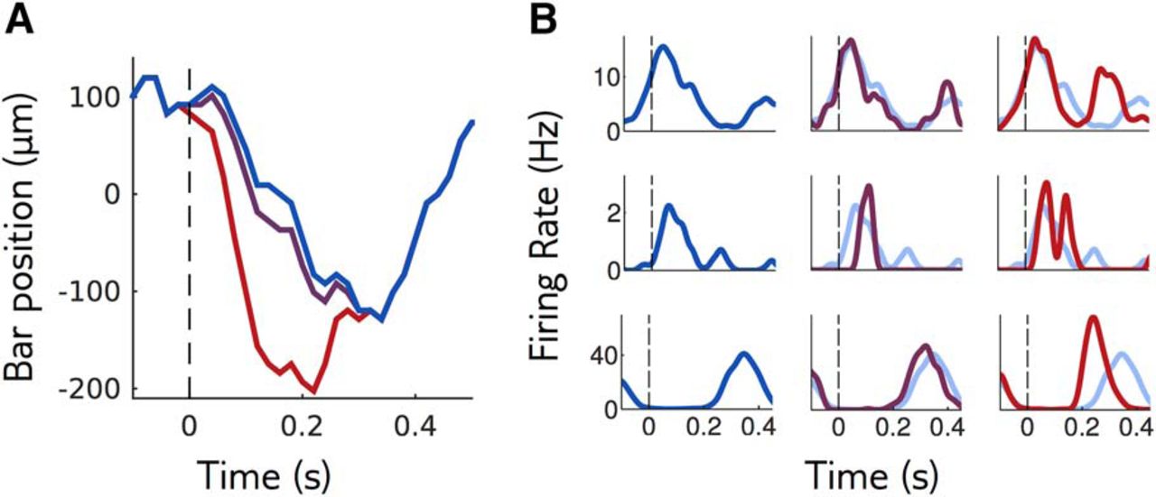


