

Abstract
Humans instantly recognize a previously seen face as “familiar.” To deepen our understanding of familiarity-novelty detection, we simulated biologically plausible neural network models of generic cortical microcircuits consisting of spiking neurons with random recurrent synaptic connections. NMDA receptor (NMDAR)-dependent synaptic plasticity was implemented to allow for unsupervised learning and bidirectional modifications. Network spiking activity evoked by sensory inputs consisting of face images altered synaptic efficacy, which resulted in the network responding more strongly to a previously seen face than a novel face. Network size determined how many faces could be accurately recognized as familiar. When the simulated model became sufficiently complex in structure, multiple familiarity traces could be retained in the same network by forming partially-overlapping subnetworks that differ slightly from each other, thereby resulting in a high storage capacity. Fisher’s discriminant analysis was applied to identify critical neurons whose spiking activity predicted familiar input patterns. Intriguingly, as sensory exposure was prolonged, the selected critical neurons tended to appear at deeper layers of the network model, suggesting recruitment of additional circuits in the network for incremental information storage. We conclude that generic cortical microcircuits with bidirectional synaptic plasticity have an intrinsic ability to detect familiar inputs. This ability does not require a specialized wiring diagram or supervision and can therefore be expected to emerge naturally in developing cortical circuits.
Significance Statement
Humans recognize familiar faces instantly. The cellular mechanisms underlying this recognition memory are still poorly understood. Simulations presented here demonstrate that bidirectional synaptic plasticity is sufficient to endow recurrent spiking neuronal network models with the ability to detect familiar sensory inputs through unsupervised learning. Network spiking activity evoked by a face image results in changes in synaptic connectivity and the formation of a unique strengthened subnetwork. Networks can recognize multiple previously seen faces with high accuracy by forming partially overlapping subnetworks. We therefore propose that familiarity detection is an intrinsic property of generic cortical microcircuits with bidirectional synaptic plasticity.
Introduction
Recognition memory refers to the ability to recognize previously experienced sensory inputs. Prior studies (Nickerson, 1965; Shepard, 1967) found that immediately following a single exposure to 612 pictures, subjects could select the previously-seen picture in two-alternative recognition tests with 98% accuracy. Later, Standing (1973) reported that the number of pictures correctly recognized increases with the number of pictures presented (up to 10,000), suggesting a limitless capacity of recognition memory. These experimental observations can be accounted for by familiarity, a form of unsupervised learning. Familiarity and recollection are two major processes that underlie recognition memory (Yonelinas, 2002; Squire et al., 2007). While recollection demands accurate recall of the object’s features, familiarity merely requires a signal indicating that the object has been previously encountered (Wixted, 2007). Evidence from functional imaging studies shows that cortical regions surrounding the hippocampus become active when a human subject senses a familiar input, whereas activation of the hippocampus is required for recollection (Hölscher et al., 2003; Diana et al., 2007).
While learning and memory have been extensively studied at the molecular/cellular (Wu et al., 2006; Baudry et al., 2015) and behavioral (Gale et al., 2014; Rapanelli et al., 2015) levels, it has been difficult to causally connect these two levels of desciption (Morgado-Bernal, 2011). Memories are believed to be encoded by and stored in a subset of neurons (the “engram”), which are connected by synapses whose weights were altered by the learning experience (Takeuchi et al., 2014). Given the current knowledge on how learning induces changes in synaptic efficacy through long-term potentiation (LTP; Bliss and Lomo, 1973), long-term depression (LTD; Ito and Kano, 1982; Massey and Bashir, 2007), and spike-timing-dependent plasticity (STDP; Gerstner et al., 1996; Markram et al., 1997; Bi and Poo, 1998), it is meaningful to simulate the synaptic changes in biologically plausible neural networks, to foster understanding from a systems perspective.
The liquid state machine (LSM) is a biologically-inspired spiking neural network model, which closely emulates the complexity of a generic cortical microcircuit. It is designed to perform biologically realistic real-time computing on time-varying inputs, providing an alternative to the widely-used attractor neural networks which require convergence to stable internal states (Maass et al., 2002). The construction of an LSM network, which involves generating random connections with random synaptic weights, is task independent. An important property of these networks is that sensory inputs are expanded into high-dimensional feature space, allowing linear separation of complex properties (Buonomano and Maass, 2009). Temporal and spatial input information is transiently preserved in the form of fading memory, through multiple recurrent loops and short-term synaptic plasticity (depression and facilitation). We have introduced activity-dependent long-term synaptic plasticity into the network model by incorporating NMDA receptor (NMDAR) functionality (Shouval et al., 2002) in the excitatory synapses.
NMDARs are critically important for synaptic plasticity-dependent learning. When post-synaptic depolarization coincides with glutamate and glycine binding, NMDARs open and allow Ca2+ influx (Blanke and VanDongen, 2009). Depending on the amount of Ca2+ influx, it will selectively activate phosphatases (low calcium influx) or the kinase CaMKII (high calcium influx), and trigger downstream signaling for synaptic depression or potentiation, respectively (Salter et al., 2009; Malleret et al., 2010; Luscher and Malenka, 2012), a theory known as the calcium control hypothesis (Lisman, 1989). LTP and LTD can be induced by tetanic synaptic inputs that regulate the Ca2+ influx. They are rate-based: low-frequency stimulation causes LTD, while a high-frequency tetanus induces LTP. STDP is another form of synaptic plasticity regulated by the temporal correlation of pre- and post-synaptic firing. By implementing back-propagating action potentials (BPAPs), NMDAR functionality can support STDP through calcium control (Waters et al., 2005; Paradiso and Wu, 2009). We have implemented both rate-based (LTP/LTD) and spike-timing-based (STDP) plasticity, by modeling NMDAR functionality in the excitatory synapses using the calcium control hypothesis.
The NMDAR-containing neural network is a model of generic cortical microcircuits with the capability of unsupervised learning. We have used it here to study how familiarity could develop in the cortex. On a large scale, brain regions are wired into relatively deterministic neural circuits (Coutlee and Huettel, 2012; Fornito et al., 2012), yet randomness and flexibility prevails within local cortical regions, with functional connections being optimized by activity-dependent changes (Sporns and Zwi, 2004; Fair et al., 2009). The main hypothesis underlying our simulations is that a sensory stimulus induces changes in synaptic weights in a neural microcircuit, altering the network response such that it can distinguish familiar from novel inputs.
Materials and Methods
Neural network implementation
Neural networks were simulated using MATLAB and the CSIM package (a neural Circuit SIMulator, RRID: SCR_014256, available at http://www.lsm.tugraz.at/csim/), as described previously (Natschläger et al., 2002; Ju et al., 2013). NMDAR-dependent synaptic plasticity was introduced into the excitatory synapses following the model proposed by Shouval et al. (2002). The neural networks consist of two parts: an input layer, and the network reservoir. Input neurons send spikes to the network reservoir via static spiking synapses, which have no plasticity. The network reservoir consists of leaky integrate-and-fire (LIF) neurons recurrently connected by NMDAR synapses. Seventy-five percent of the neurons are set as excitatory, the remaining being inhibitory. Each LIF neuron is modeled by a linear differential equation: (1)where the parameters are: membrane time constant τm = 30 ms, Vresting = 0 mV, membrane resistance Rm = 1 MΩ, input currents supplied by explicitly modeled synapses Isyn, steady background current Iinject = 13.5 nA and for some simulations random noise Inoise was added to the current. For the first time step in the simulation, the membrane potential Vm was set to an initial random value between −1 and 1 mV. When Vm increases to 15 mV (the firing threshold), the neuron fires, and Vm is reset to a random value between −1 and 1 mV after an absolute refractory period of 3 ms for excitatory neurons and 2 ms for inhibitory neurons (Joshi, 2007).
In CSIM, the probability that two neurons are connected by a synapse is defined as: (2)where D(a,b) stands for the Euclidean distance between the two neurons a and b. λ and C are parameters used by CSIM that determine connectivity and synaptic strength, respectively. As λ increases, both the connection probability and the average connection length will increase. The base value of C depends on the type of connection: it is set to 0.3, 0.2, 0.4, and 0.1 for EE, EI IE, and II connections, where E and I stand for excitatory and inhibitory neurons. The values are based on recordings from rodent cortical brain areas (Gupta et al., 2000). The actual value of C is modulated by a user-defined parameter, Cscale. Input layer neurons are all excitatory. Connections from input neurons to the network reservoir and within the network reservoir are randomly generated following the probability P(D).
Once a connection is established, it is assigned an initial synaptic weight, indicating synaptic efficacy. Initial synaptic weights are drawn from the following gamma distribution: (3) where Γ (·) is the Gamma function. SH_W and W are parameters used by CSIM. SH_W (default 0.7) positively correlates with the variance of the weight distribution and W correlates with the mean of the distribution. The base value of W is set to 3e−8 for EE, 6e−8 for EI, −1.9e−8 for IE and II. The actual value of W is modulated by a user defined parameter, Wscale. The synaptic weight of an excitatory NMDAR synapse is subject to strengthening (upper boundary = 6.5e−8) or weakening (lower boundary = 1.0e−9) by plasticity. Synapses from the inhibitory neurons have negative weights, and do not possess plasticity. Synaptic weights of the static spiking synapses from input neurons are fixed.
In CSIM, a network is generated by placing neurons on a 3-D grid. The networks described in Figure 1A had five layers with 10 × 10 neurons each (dimension, 10 × 10 × 5). Input neurons formed synapses one-to-one with the first layer of the network reservoir, with fixed synaptic weights of 2.7e−7. NMDAR synapses in the network reservoir were generated with λ = 2.0 and Cscale = 1.0. Initial weights followed the gamma distribution with SH_W = 0.25 and Wscale = 0.5.

Network architecture and stimulus encoding. A, Diagram illustrating a 10 × 10 × 5 network with a 10 × 10 input layer, receiving a stimulus from a beard face image (10 × 10 pixels). Neurons in the network reservoir are located at positions with integer coordinates in a 3-D space. The input layer is located 1 unit away from the network reservoir. Input neurons form synapses one-to-one with the first layer of the network reservoir. Each input neuron receives a spike train with a firing rate determined by the corresponding image pixel intensity value. B, Diagram illustrating a 50 × 50 × 5 network (only a portion of size 15 × 15 × 5 is shown) with a 50 × 50 input layer (only 15 × 15 portion is shown), receiving a stimulus from a human face image (50 × 50 pixels). Input neurons form synapses with random neurons in the network reservoir. C, Examples of a 10 × 10-pixel beard face (top) and a 10 × 10-pixel no-beard face (bottom). D, Examples of 20 × 20-pixel images of car fronts, dog faces and human faces. E, Examples of 50 × 50-pixel human faces. F, A sample beard stimulus which contains spike trains (0–0.5 s), followed by a silent interval (0.5–1.0 s). Only 50 channels of spike trains are shown for clarity.
Networks described in Figure 1B consisted of five or six layers, with dimensions 20 × 20 × 5, 50 × 50 × 5, and 50 × 50 × 6. In this case, input neurons formed synapses randomly with the network reservoir with Cscale = 0.04, 0.004, and 0.005, respectively, and λ was set to infinity in all cases to remove the limitation by distance. As a result, there was no topographical mapping of the input pattern. Input synaptic weights were still fixed but no longer uniform, following a gamma distribution (Wscale = 3, SH_W = 0.7 in all cases) instead. As for NMDAR synapses in the network reservoir, λ = 4.0 for the 20 × 20 × 5 networks; λ = 3.0 for 50 × 50 × 5 and 50 × 50 × 6 networks; Cscale = 1 for all cases. The λ values were chosen to make sure that each neuron formed ∼100 synapses on average with others in the network. Initial weights of NMDAR synapses also followed a gamma distribution with Wscale = 0.9 and SH_W = 0.25. By setting Wscale to 0.9, the initial weights were set to intermediate values, leaving enough room for future potentiation and depression. By setting SH_W to 0.25 for the network reservoir, we reduced the variation in the initial weights, thereby reducing any preimposed network circuitry.
Synaptic plasticity implementation
The NMDAR-dependent plasticity we implement follows the model by Shouval et al. (2002). Synaptic plasticity (LTP/LTD and STDP) depends critically on the amplitude and timing of postsynaptic EPSPs and BPAPs. BPAPs were not implemented in the original CSIM, while EPSPs were implemented using a single exponential decay function with a time constant of 3 ms. We introduced BPAPs and changed both BPAPs and EPSPs to follow double-exponential decays, each with a fast and a slow component. Decay time constants were scaled from the suggested values (Shouval et al., 2002), with BPAP fast decay time constant  = 1.2 ms and proportion
  = 0.75, slow decay time constant
  = 10 ms and proportion
  = 0.25; EPSP fast decay time constant
  = 2 ms, proportion
  = 0.5, slow decay time constant
  20 ms and proportion
  = 0.5.
 (4)
(4)
 (5)
(5)
Using a double-exponential decay ensures that the BPAP has a sharp peak with a thin tail and that the EPSP has a slower peak and more prominent tail, thereby preserving the difference in temporal signature between EPSPs and BPAPs. This contrast ensures that the change in intracellular Ca2+ concentration induced by pre-post firing exceeds the [Ca2+] change induced by post-pre firing, so that STDP will be induced properly (see Fig. 2 in Shouval et al., 2002).
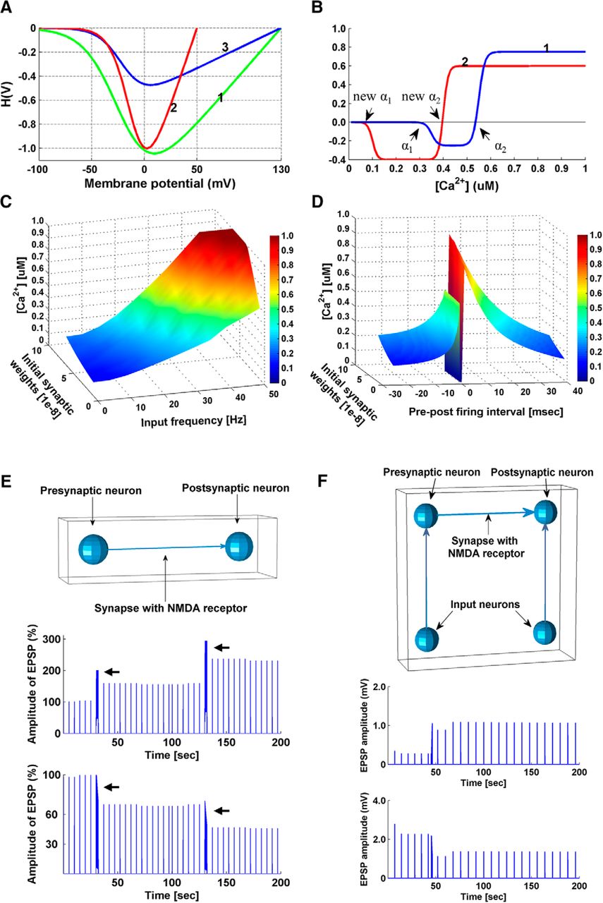
Parameter turning. A–D, Calcium control hypothesis. A, Curves illustrating the driving force function H(V): (1) as proposed in (Shouval et al., 2002); (2) from in vitro recordings of ion currents through NMDARs (Pattillo et al., 1999); (3) re-parameterized in our model. Curve (3) is similar to (2) at negative membrane potentials. Curve (3) has the same equilibrium potential as (1) but is smaller in amplitude, reducing the impact of growing synaptic weights. B, Models of the calcium control hypothesis Ω function: (1) as proposed in (Shouval et al., 2002), (2) as used in our simulations. When real-time synaptic Ca2+ concentration ([Ca2+]) exceeds the new α1 but not the new α2, synaptic weight is decreased; when real-time synaptic [Ca2+] exceeds the new α2, synaptic weight is increased. C, Real-time postsynaptic [Ca2+] is plotted as a function of input frequency and initial synaptic weights. D, Real-time postsynaptic [Ca2+] is plotted as a function of pre-post firing intervals and initial synaptic weights. E, Induction of LTP/LTD at individual synapses following high/low-frequency stimulation protocols. Top, Model setup. A presynaptic input neuron is connected to a postsynaptic neuron by an excitatory NMDAR synapse. The presynaptic input neuron generated spikes at a certain frequency, and EPSPs were recorded in the postsynaptic neuron. The postsynaptic neuron is prevented from firing action potentials. Middle, Simulation results with 50 Hz tetanus input on the model. Spike trains of 50 Hz were generated by the presynaptic input neuron, which caused long-lasting increases of the EPSP amplitude in the postsynaptic neuron. Arrows indicate when a 50 Hz tetanus (2 s) was applied. Bottom, Simulation results with 20 Hz tetanus input on the model, which resulted in a long-lasting decrease in the amplitude of EPSPs. Arrows indicate when a 20 Hz tetanus (2 s) was applied. Results are comparable to observations from Bliss and Lomo (1973) and Ito and Kano (1982). Baseline spikes at a frequency of 0.2 Hz were generated by the presynaptic input neuron, in addition to the tetani, to probe the changes in EPSP amplitude. F, Simulation of a dual patch clamp STDP experiment. Top, Model setup. A presynaptic neuron is connected to a postsynaptic neuron by an excitatory NMDAR synapse. EPSPs were recorded in the postsynaptic neuron. Two input neurons are connected to the pre- and post-synaptic neurons to control their firing time. STDP simulation results are comparable to observations of STDP in cortical neurons (Froemke et al., 2010). Middle, Potentiation was induced in the model by pre-post firing (Δt = 15 ms, 15 pairings). Bottom, Depression was induced by post-pre pairing (Δt = −75 ms, 30 pairings). Baseline spikes were generated at a frequency of 0.125 Hz by the input neuron connected to the presynaptic neuron to probe the changes in EPSP amplitude.
Activity-induced EPSPs generate the driving force for calcium currents through the NMDAR: (6)where V = Vresting + EPSP + BPAP, and Vr is the reversal membrane potential for calcium (130 mV). The Mg2+ concentration is set to 1 mM. The driving force function was modified from the function suggested by Shouval et al. (2002) which did not take into consideration the effect of growing synaptic weights. In vitro recordings of ion currents through NMDARs (Pattillo et al., 1999) show a steeper curve, and based on this, we re-parameterized the calcium driving force (Fig. 2A).
The calcium current through NMDARs ( ) is assumed to have this form:
 (7) where PO is the probability of opening, G is the conductance of the NMDAR channel, If and Is are the fast and slow components of the NMDA currents, τf and τs are the time constants for the fast and slow components.
Calcium control hypothesis
The activity-dependent change in synaptic calcium concentration is modeled as a function of the NMDA current  :
: (8) where
  is the calcium concentration at the synapse at time t and
  is the decay time constant, which is assumed to be 50 ms. The weights of NMDAR synapses are modified by calcium concentration as follows:
 (9)
(9)
The Ω function represents the calcium control hypothesis with α1 and α2 being [Ca2+] thresholds for depression and potentiation induction: (10)
(10)
The parameter values were originally set as follows: α1 = 0.35 µM, α2 = 0.55 µM, β1 = β2 = 80 µM, and  = 0.25 (Shouval et al., 2002). By setting new α1 to 0.1 µM and new α2 to 0.4 µM (Fig. 2B), we were able to induce LTD at low input frequency (1–20 Hz) and post-pre firing (−15 ∼ −5 ms) regardless of the synaptic weights, while LTP was obtained at high input frequency (50–100 Hz) and pre-post firing at (5 ∼ 15 ms), regardless of the synaptic weights (Fig. 2C,D; Table 1). We also changed
  from 0.25 to 0.4, rendering the plasticity more biased toward LTD to stabilize network activity after prolonged sensory exposure.
Postsynaptic Ca2+ concentration [µM]
Individual synapse performance
After parameter tuning described in the sections above, we simulated the classic tetanus experiment (Bliss and Lomo, 1973) and dual patch clamping experiment (Markram et al., 1997) on single NMDAR synapses. The synaptic efficacy change successfully reproduced previously published results (Fig. 2E,F), indicating the reliability of our model at individual synpase level.
Image preprocessing
For the beard versus no-beard classification simulations, grayscale images of male faces with and without a beard were selected to form two groups, 20 images for each group. Each image was reduced to a 10 × 10 pixel pattern (Fig. 1C). For the single face recognition simulations, we used grayscale images of car fronts, dog faces and human faces, 10 images for each category. Each image was converted to a line drawing using edge detection to reduce noise from shading and then down-sampled to a 20 × 20 pixel pattern (Fig. 1D). For the multi-face recognition simulations, 200 grayscale human face images were selected and each face image was converted to a line drawing and down-sampled to 50 × 50 pixels (Fig. 1E). Images were presented to the network by assigning each pixel to a corresponding input neuron and converting pixel values to spike trains. Grayscale values of 0–255 were mapped to frequencies of 0–50 Hz. Each image stimulus lasted 0.5 s, followed by a silent interval of 0.5 s (Fig. 1F) to allow the fading memory to dissipate and prepare the network for the next stimulus.
Fisher’s discriminant analysis
Multiclass Fisher’s discriminant analysis was applied to network spiking activity and neuronal spiking activity, to obtain Fisher’s linear discriminant ratio (FDR). The FDR is calculated as follows: (11)where
  is the spike count at time bin t, in response to stimulus i;
  is the mean spike count at time t for class C stimuli, and
  is the mean of the class means
  . The numerator and denominator of the discriminant ratio J are known as the “between classes scatter” and “within class scatter.” A larger value of J indicates better discrimination. More information can be found in Ju et al. (2015).
Network FDR was obtained by summing up the FDRs calculated with network spiking activity in each time bin, serving as an indicator of network separability for input stimuli. Neuronal FDR was calculated with the spiking activity of individual neurons over the entire recording period, serving as an indicator of how informative the neuron is for input discrimination.
Results
We performed simulations of cortical microcircuits modeled with NMDAR-containing neural networks (see Materials and Methods), to investigate whether they can develop recognition memory. Images were used as sensory inputs and plasticity was enabled during learning and disabled during evaluation of responses to the input images. Simulations typically consisted of three phases: baseline recording, learning and testing. First, to establish a baseline, network responses to all input stimuli were recorded while NMDAR function was disabled. Network firing rate (spikes/second) during the stimulus presentation was calculated and used as a measure of network response. In the second phase, learning was switched on by enabling NMDAR plasticity, and networks were stimulated using only a subset of images, allowing stimulus-induced network spiking activity to alter synaptic strengths. These images should now be “familiar” to the networks. Finally, learning was switched off and network responses to all input stimuli were recorded again. The effect of the learning experience was evaluated for both familiar images presented during the learning phase and the “novel” images, by comparing testing responses with their corresponding baseline values. In all of our simulations, we found that the networks responded differentially to images presented during the learning phase.
Unsupervised classification: beard versus no-beard
In this first set of simulations, two classes of images were used: human faces of males with and without a beard. In each simulation, only faces from a single class (beard or no-beard) were presented to a network during the learning phase. In each learning round, one face from the selected class was randomly chosen and presented to the network for 1 s. NMDAR plasticity was switched off for testing after each round, and network responses to all faces from both classes were recorded. Figure 3A summarizes the performance of five randomly-generated 10 × 10 × 5 networks for 40 rounds of image presentation. Clearly, networks responded more strongly to faces from the trained class, and the firing rate discrepancy for the two classes increased as more faces were presented. In other words, networks started to display a differential response to the two classes as unsupervised learning took place. This was true whether the beard or no-beard class was used for training. The differential response eventually reaches a steady state, in part because we have set a maximum weight boundary (6.5e−8) for excitatory synapses to prevent overtraining. We also investigated network performance by excluding faces that were presented in the learning phase from the testing. The results showed a similar increase in discrepancy for the responses to the two classes, only with a reduced magnitude (Fig. 3A). In this case, the networks were performing a binary classification task, following unsupervised learning.

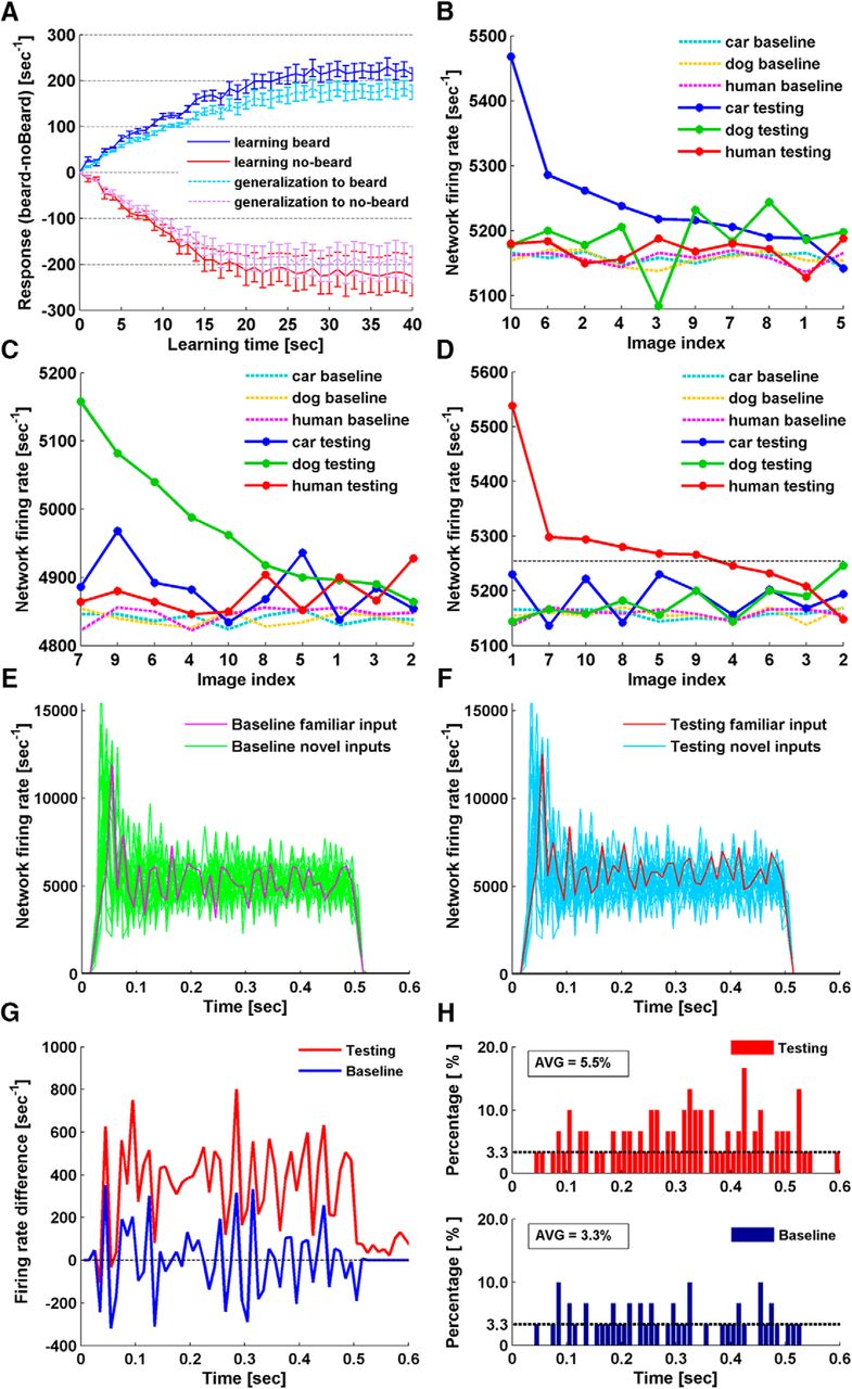
Unsupervised familiarity detection. A, Beard versus no-beard classification. Curves showing the discrepancy in network responses (firing rate [sec−1]) to beard and no-beard faces that develops with sensory exposure to one class. The blue curves represent network response (beard-noBeard) after learning beard faces. The dark blue solid line shows response differences when trained beard faces were used for testing. The light blue dashed line shows the results when untrained beard faces were used for testing, i.e., networks generalizing familiarity to novel beard faces. The red curves represent the results from the same simulation paradigm with no-beard faces used for learning. The red solid line shows response differences when trained no-beard faces were used for testing. The pink dashed line shows the results when untrained no-beard faces were used for testing, i.e., networks generalizing familiarity to novel no-beard faces. Error bars at each time point reflect the SEM of results from five randomly-generated networks. Each network underwent five trials of simulation with randomly-selected face inputs. Curves were normalized by subtracting the discrepancy of network baseline response to the two classes at time 0. B–D, Single face recognition. B, The network test responses (solid lines) and corresponding baseline responses (dashed lines) to all 30 images after learning car image 10. Test responses to car images were sorted in descending order. As images of each class were indexed as 1–10, test responses to the other two classes are plotted following the sorted index order. C, Network responses to all 30 images after learning dog image 7. D, Network responses to all 30 images after learning human face 1. E, F, Firing rate dynamics during stimulus presentation of the network shown in D. E, Network baseline firing rate to all 30 stimuli. F, Network firing rate to all 30 stimuli after learning human face 1. The stimulus of human face 1 is referred as the familiar input. G, Firing rate difference between response to the familiar input and the average of the responses to the novel inputs. The average performance of 10 networks in 30 simulations has been shown. Blue represents the difference in network baseline responses. Red represents the difference in network testing responses, after the single face recognition simulations. H, Histograms of time bins where the networks exhibited the highest firing rate to the familiar input. Network firing rate was obtained as in E, F, binning was at 10 ms. Time bins where networks exhibited the highest firing rate to the familiar input were identified. The number of the identified time bins was summed for 30 simulations carried out 10 networks, and the percentage was calculated with respect to 30 simulations, with chance level being 1/30 (3.3%).
Single face recognition
Next, we performed single face recognition simulations, for which we increased the dimension of the networks to 20 × 20 × 5 and the input layer size to 20 × 20. A set of 30 images was used as input stimuli, consisting of 10 car fronts, 10 dog faces, and 10 human faces. The simulations again consisted of three phases: baseline normalization, learning, and testing. NMDAR-dependent plasticity was only switched on during the learning phase. Normalization was performed by recursively adjusting the mean pixel value for each of the 30 images until they evoked comparable baseline responses. In the learning phase, a single human face image was selected from the set of 10, and presented repetitively for 15 s. NMDAR-dependent plasticity was then switched off for the testing phase, in which we recorded network responses to all images, to determine whether the network responded differently to the selected (learned) face.
For this simulation, we used 30 randomly-generated networks. Instead of limiting the stimuli to human faces, we also conducted trials using images of car fronts and dog faces. For each network, three trials were conducted, each with a randomly selected car, dog, or human image. In total, 90 trials were performed on the 30 networks, and in 84 cases (93.3%), the networks exhibited the highest firing rate to the image presented during the learning phase. Examples of network responses before and after the learning phase are shown in Figure 3B–D. Testing responses are sorted by firing rate and shown as solid lines, while corresponding baseline responses are plotted as dashed lines. Network firing rate to the images selected for learning significantly increased and became the largest on testing. Responses to novel inputs from the same class as the image selected for learning tended to be elevated from their baseline, although to a lesser extent than the actual learned image. For instance, in the human face learning simulation (Fig. 3D), the network responses to 5 of the 10 human faces (excluding the learned face) were higher than the responses to the dog and car images, suggesting that the network had also generalized to distinguish human faces from dog faces and car fronts. Considering the degree of randomness involved in network construction, and the similarity of the images within each class, we conclude that networks of 20 × 20 × 5 neurons can learn to detect a familiar image with high specificity.
The network responses in Figure 3B–D are network firing rates averaged over the entire recording period. In fact, the dynamic network firing rates plotted as a function of time underwent initial rising phases and declined to steady state phases (Fig. 3E,F). By solely looking at firing rate difference, network response to the familiar input seems to have increased over the entire recording period after learning (Fig. 3G). Whether the increase in individual time bins is sufficient for familiarity detection is further analyzed. If we assume the networks are able to detect familiarity in the time bins where networks exhibited the largest firing rate to the familiar input, we can count the number of such time bins and compare it before and after learning. The results show that there is no specific time window that clearly separates the familiar input from the novel inputs, but the separation gets better in the later stage of stimulus presentation (Fig. 3H).
Multi-face recognition
Now that these relatively small neural networks have demonstrated they can discriminate a single familiar face from many novel ones, we tested whether networks can perform familiarity detection to more than one face. We began with presenting two human face stimuli to a single network, using the same set of 30 images and 20 × 20 × 5 networks. Unlike the high accuracy (93.3%) of the single face recognition simulations, familiarity detection accuracy for two face stimuli dropped to 70.0% (data not shown). This performance decline informs us of the limited capacity of 20 × 20 × 5 networks.
We therefore increased dimensions of the networks to 50 × 50 × 5 and input layers size to 50 × 50. In addition, the resolution of the 30 images was increased to 50 × 50 pixels, so that their dimension matched that of the input layer. With these larger networks, the accuracy of familiarity detection for two face stimuli increased to 96.7%. The performance improvement could be due to either the increase in network size or the increase in resolution of the face images. To distinguish between these two options, we repeated the simulations on 50 × 50 × 5 networks, but with the original low-resolution 20 × 20 pixel image stimuli as inputs. Each pixel in the 20 × 20 images was replicated once to create images of 40 × 40. One column and one row of void pixels were then added to the right and bottom of the matrices to make images of dimension 50 × 50. When these low-resolution 50 × 50 stimuli were presented to the networks, the accuracy of familiarity detection remained at 96.7% (Fig. 4A), suggesting that increased network dimension was responsible for the accuracy improvement.

Familiarity detection for multiple faces. A, Results of 50 × 50 × 5 networks learning two human faces. Each bar is located at the point whose coordinates represent the rank of network firing rate for the two learned faces. The height of each bar reflects the number of occurrences of such a combination (30 in total). Blue and magenta represent network baseline and testing response, respectively. Note that after learning, the two familiar faces ranked 1 and 2 in 29 of 30 trials and 1 and 3 in the remaining trial. B–E, Results of learning 10 faces and testing them against 10 novel faces randomly drawn from a database of 200 faces. B, Results of a 50 × 50 × 5 network learning 10 faces. The curves show baseline and sorted testing response after learning faces 1–10. The network ranks nine familiar faces among the top 10, with only one outlier (face 62, highlighted in magenta). The accuracy of this network therefore was 9/10 or 90%. C, The effect of network dimension and Cscale value was evaluated by performing 1000 trials for 10 different networks (see Results). For each trial, the accuracy was calculated as in B. The curves illustrate the accuracy (averaged over 1000 trials) for the 10 networks with dimensions and Cscale values indicated in the legend. D, Accuracy distribution of 1000 testing trials conducted on the ten 50 × 50 × 6 networks with Cscale 0.005. E, Baseline and testing response of the best-performing 50 × 50 × 6 network after learning face 1–10. Network firing rate differentiates familiar faces completely from novel faces. F, Network average accuracy of the 50 × 50 × 6 networks after learning 10 faces (red) and the corresponding accuracy after learning 30 faces (green), 60 faces (blue), and chance level at 60 faces (gray, dotted line). Error bars are the SDs of 1000 trials. G, top, Baseline and testing response of the best-performing 50 × 50 × 6 network to all 200 faces and their scrambled versions, after learning face 1–10. F, faces; SF, scrambled faces. Bottom, Pairwise network firing rate difference to faces and scrambled faces (F-SF).
Interclass learning of three image classes (car + dog + human) using 50 × 50 × 5 networks also produced stable and accurate results (data not shown). For multiple images, we presented each image for 15 s and then moved to the next image. In contrast, we also tried looping through all images 15 times. The first presentation protocol resulted in slightly better accuracy, and was used for all the remaining simulations.
To further evaluate the limits of these neural networks on multi-face recognition, we converted a database of 200 human face images to 50 × 50 pixel stimuli. In each simulation, a randomly-generated 50 × 50 × 5 network was presented with 10 human face images, each for 6 s, and testing was conducted with the 10 learned faces plus 10 novel faces drawn randomly from the database. We used 6 s instead of 15, to prevent overtraining of the network. After sorting the network firing rate for all 20 faces, a hypothetical threshold was drawn between the responses to faces ranking 10th and 11th, to evaluate the ability of the networks to separate familiar and novel faces. This procedure is similar to the empirical ranking theory of vision (Purves et al., 2011), which suggests that subjects perceive the relative color and brightness of objects by internally ranking the empirical brain activity they evoke. In our case, the percentage of learned faces appearing in the top 10 reflects familiarity detection accuracy. The 10 faces used for presentation to the networks were randomly selected from the database, indexed as 1–10 and fixed for all simulations. The 10 novel faces were randomly drawn from the remaining database and were varied for each testing trial. Figure 4B shows the sorted responses and hypothetical threshold for a network that was able to detect 9 out of the 10 presented faces in one testing trial, and therefore was considered 90% accurate for this trial. The average accuracy of a network was measured by averaging the results of 1000 testing trials. Performance of ten randomly-generated 50 × 50 × 5 networks for the above simulations is shown in Figure 4C, blue. The best network reached ∼85% accuracy on average for 10-face familiarity detection.
In an attempt to further improve the performance, we generated a different set of ten randomly-generated networks, with one more layer added to the network reservoir (50 × 50 × 6), and increased the connection probability from the input layer to the reservoir (Cscale = 0.004 to Cscale = 0.005). The resulting network average accuracy is shown in Figure 4C, red. Not only did the overall accuracy improve, but also a network with >95% accuracy emerged, indicating the network was able to detect all 10 familiar faces accurately for at least half of the 1000 testing trials. Figure 4D summarizes the accuracy distribution of 1000 testing trials for the ten 50 × 50 × 6 networks. The distribution is significantly shifted from what would be expected by chance alone, i.e., five familiar faces falling in the top 10. Figure 4E plots the response of the best-performing 50 × 50 × 6 network for one of the testing trials. Unsupervised learning has clearly modified the network response and a hypothetical threshold can be drawn which accurately differentiates familiar from novel faces.
We also evaluated the performance of ten randomly-generated 50 × 50 × 5 networks with Cscale 0.005 and ten randomly-generated 50 × 50 × 6 networks with Cscale 0.004 (Fig. 4C, dotted lines). Neither achieved comparable accuracy as 50 × 50 × 6 networks with Cscale 0.005. From these results, it seems that both the network size and the number of input connections are important. An increase of input connections together with a larger network results in larger available network space for better familiarity storage.
In fact, the network capacity of multi-face recognition is not restricted to 10 faces. In Figure 4F, we plot the accuracy of the ten 50 × 50 × 6 networks after learning 10 faces (red), 30 faces (green), and 60 faces (blue), as well as the chance level for 60 faces (gray). To our surprise, only two networks performed equivalently to or below their corresponding chance levels after learning 60 faces. The remaining eight networks performed significantly better than chance levels (Table 2, n = 1000, p < 0.01). Accuracy after learning 30 and 60 faces was measured by the percentage of familiar stimuli appearing above the hypothetical threshold (set as below 50% of the population) after pooling the same number of novel stimuli with familiar stimuli. The chance level at 60 faces was calculated by the percentage of familiar stimuli appearing above the hypothetical threshold after sorting network baseline firing rates to the familiar and novel stimuli.
Statistical table
In addition, we generated scrambled versions of the 50 × 50 face images from the same database by relocating all pixels to new random (x, y) positions, and recorded the network responses to them after learning 10 human faces. The results show that networks not only discriminated the familiar faces from the novel faces, but also could discern novel faces from their scrambled versions (Fig. 4G). The trained networks appeared to have acquired the concept of a “face” and responded less to scrambled faces.
Synaptic weight change
Given that synaptic weight changes underlie the observed results described above, we plot in Figure 5 the network weight changes in three scenarios: weight change after exposure to a human face stimulus for 1, 3, and 5 s (Fig. 5A); weight change after exposure to a car, a dog or a human face image each for 15 s (Fig. 5B); and weight change after exposure to multiple face images (Fig. 5C). A common finding emerges for all three scenarios: unsupervised learning caused a subset of synapses to be potentiated, and a different but larger subset of synapses to be depressed. The amplitude of potentiation is larger than the amplitude of depression, on average. This is in line with a proposed familiarization mechanism that a small subset of neurons becomes strongly responsive after sensory exposure while depression occurs pervasively among other neurons, sharpening the familiarity response (Freedman et al., 2006; Meyer et al., 2014). Figure 5D shows the time course of the change in synaptic strength for nine representative synapses randomly picked from a 50 × 50 × 6 network during the exposure to 10 faces. Synaptic weights changed in unique ways in response to each face stimulus.

Synaptic weight changes caused by learning. A, Network synaptic weight change after the presentation of 1, 3, and 5 s of the same human face stimulus, in comparison to initial synaptic weights. B, Network synaptic weight change after learning a car, dog, or human stimulus, each for 15 s, in comparison to initial synaptic weights. C, Network synaptic weight change after learning 1, 5, and 10 human face image stimuli, each for 6 s, in comparison to initial synaptic weights. A–C, Only a subset of NMDAR synapses in the network are shown for clarity and the y-axis scales are ±1e−7. D, Time course of weight change of nine randomly-selected NMDAR synapses during the exposure to ten faces, each for 6 s.
Subnetwork formation
If we put together the phenomena of how synaptic weights change after sensory exposure and how available network space affects accuracy, a theory emerges that could possibly address the stability-plasticity dilemma (Grossberg, 1980, 2013; Mermillod et al., 2013). Whenever a new image stimulus enters the network reservoir, an image-representative subnetwork is formed by potentiated and depressed synapses. Providing the network reservoir is large enough and has sufficient complexity, a large number of image-representative subnetworks that differ slightly from each other can co-exist in the network. This reduces the chance that formation of a new memory overwrites an older one, allowing each subnetwork to support familiarity detection. To provide support for this idea, we identified the set of synapses whose weights were modified after the stimulus presentation. In Figure 6A,B, the potentiated synapses are highlighted in red and green, respectively, for the same network after exposure to two different face images. In Figure 6C, the potentiated synapses are highlighted after the same network was exposed to both face images. Notice the difference between the two image-representative subnetworks, and how they can co-exist in the network reservoir. These subnetworks may act as neural clusters carrying memory traces (Liu et al., 2012). In Figure 6A–E, the subnetworks are viewed from the top. As the faces resemble each other to a certain degree, the corresponding subnetworks are proximate to each other. They are also densely connected through the layers, as seen in a side view (Fig. 6F).

Importance of subnetwork topology. A–C, Colored lines indicate potentiated synaptic connections of a 50 × 50 × 6 network after learning face 1 (A), face 2 (B), or face 1 and 2 (C). Yellow highlights the synapses in C that also appeared in both A and B; red and green highlights the synapses that only appeared in A and B, respectively. Purple indicates the synapses that newly appeared after learning both faces. D, E, Potentiated synaptic connections in the networks with the best (D) and worst (E) accuracy after learning 60 faces. F, Side views of the potentiated synaptic connections in A. G, Potentiated synaptic connections of the network in D after learning 60 faces, in comparison to synaptic weights obtained after learning 30 faces. H, Potentiated synaptic connections of the network in E after learning 60 faces, in comparison to synaptic weights obtained after learning 30 faces. I, Potentiated (red) and depressed (blue) synapses after learning face 1, for the same simulation shown in A. Thresholds for significant weight increase and decrease are 1e−8 and −1e−8 for all panels.
Following this idea, we plotted the potentiated synapses of the ten 50 × 50 × 6 networks after learning multiple faces. Figure 6D,E shows the potentiated synapses in the two networks with the best and the worst accuracy, after exposure to 60 faces (Fig. 4F, network 3 and 10, respectively). Dense clusters can be seen in the poorly-performing network (Fig. 6E). We also investigated the evolution of subnetworks from 30- to 60-face exposures. Figure 6G,H graphs the incremented subnetworks corresponding to D and E. Newly potentiated synapses are spread throughout the reservoir in the network with high accuracy, whereas newly potentiated synapses are clustered in the network with low accuracy. We calculated the average clustering coefficients (Watts and Strogatz, 1998) of the formed subnetworks for the 10 networks after learning 10, 30, and 60 faces, and correlated the average clustering coefficients with the corresponding network accuracies. The data suggest that strong clustering of subnetworks negatively affects network performance (r = −0.80, p = 9.05e−8). In general, subnetworks were more distributed in networks with better accuracy, and more aggregated in networks with poorer accuracy. One possible explanation is that overlapping subnetworks lead to increased chance for existing memories to be overwritten. The dense clustering observed in poorly performing networks might be caused by local densely-connected neurons, which tend to self-potentiate excessively due to recurrent pathways, thereby reducing memory capacity.
For the network with the best accuracy, we attempted to permute the initial weights of all NMDAR synapses of the network and repeated the same simulation of the 60-face exposure. After permutation, the network accuracy failed to remain the best. It seems that the preimposed network circuitry, which is determined by the initial synaptic connection weights, is another important factor for network performance.
Separability
In addition to using network firing rate as a readout for familiarity detection, we applied Fisher’s discriminant analysis to search for other features that may help define familiarity. Ten 20 × 20 × 5 networks and the single face recognition simulations were used for the analysis. Network response to the familiar stimulus is referred to as the familiar response, and responses to the remaining 29 stimuli are referred to as control responses. FDR is calculated between two classes (see Materials and Methods). Specifically, familiar FDR is calculated by labeling the familiar response as Class I and the control responses as Class II. Control FDRs are calculated by labeling one of the control responses as Class I and the remaining control responses together with the familiar response as Class II. Baseline FDRs are calculated in the same way but with network baseline responses to all 30 image stimuli. Baseline FDR values represent how well each image stimulus is separated from others, before learning.
Compared with the corresponding baseline FDRs, we see a general increase for both familiar FDR and control FDRs after sensory exposure (Fig. 7A). In 26 out of 30 cases, familiar FDRs show the largest magnitude of relative increase from baseline compared with control FDRs; and in 22 out of 30 cases, familiar FDRs have the largest final values. Larger familiar FDRs indicates that the network discriminated the familiar better from the control stimuli after learning, implying greater separability at the network level. Figure 7B shows the network FDRs calculated in each time bin. The larger familiar FDR can be explained by the larger FDR values in each time bin. Sensory exposure has also extended the network separability to beyond the stimulus presentation window (0–0.5 s).

FDR analysis. A–D, FDRs were calculated for the 20 × 20 × 5 network after the single face recognition simulation shown in Figure 3D. The input stimulus was human face 1, indexed as image 21 in the set of 30 test images. A, top, Network FDRs after learning human face 1. Bottom, Network FDR relative changes from baseline after learning human face 1. Red dashed lines represent the maximum in the group. Green dashed lines represent the presented stimulus. Network FDR has the largest value to the familiar stimulus after learning, and the largest relative increase from baseline. B, Network FDRs calculated with network activity in 10-ms time bins. Red lines show the FDRs to the familiar stimulus (image 21) and blue lines show the FDRs to one of the control stimuli (image 9). The filled area shows the difference between the two, with red indicating a larger value of the red line and blue indicating a larger value of the blue line. Top, The FDRs calculated based on network response after sensory exposure. Bottom, the FDRs calculated based on network baseline response. C, Neuronal familiar FDRs were calculated for the active neurons (recorded spikes > 0) after the same simulation. Top, Black indicates the sorted baseline neuronal FDRs, and red indicates the familiar FDRs of the corresponding neurons after the simulation. Bottom, black indicates the sorted baseline neuronal FDRs, and red indicates the sorted neuronal familiar FDRs. D, Baseline and testing responses to all stimuli of the neuron with the largest FDR increase in C. Red, yellow, and blue indicate responses to car, dog, and human stimuli. Neuronal baseline response is negligible, indicating an inactive role in the network. After sensory exposure, neuronal firing rate to image 21 was greatly increased. The response also generalized to other human face images (index 21–30). E, F, FDRs were also calculated for neurons in the 50 × 50 × 6 network after the simulation shown in Figure 6A. The input stimulus was human face 1 from the 200-face database. The subnetwork in Figure 6A connects 1728 unique neurons, including 187 presynaptic neurons, 1238 postsynaptic neurons, and 303 neurons that are both pre- and postsynaptic. E, Intersection of top 200 FDR neurons with the formed subnetwork (n = 118). Yellow, blue, and green indicate those FDR neurons that overlapped with presynaptic neurons (n = 26), postsynaptic neurons (n = 43), and both pre- and postsynaptic neurons (n = 49) in the subnetwork. Purple indicates nonoverlapped FDR neurons (n = 82). F, Intersection of top 200 FDR neurons calculated for control face 2 with the formed subnetwork after the network was exposed to face 1 (n = 37). Yellow, blue, and green indicate those FDR neurons that overlapped with presynaptic neurons (n = 4), postsynaptic neurons (n = 21), and both pre- and postsynaptic neurons (n = 12) in the subnetwork. Purple indicates nonoverlapped FDR neurons (n = 163).
To further understand the changes occurring at the neuronal level that supported familiarity detection, we applied the analysis to individual neurons. Similarly, familiar FDR is calculated by labeling the neuronal response to the familiar stimulus as Class I and responses to control stimuli as Class II; control FDRs are calculated by labeling the neuronal response to one of the control stimuli as Class I and responses to the remaining control stimuli and the familiar stimulus as Class II.
Compared with corresponding baseline FDRs, neurons that show increased FDRs to the familiar stimulus are considered as critical and potentially correlate with the emergence of familiarity. We noticed that the neurons with significantly increased FDRs tended to evolve more often from the neurons with negligible baseline FDRs (Fig. 7C). Neuronal baseline FDR was found to be negatively correlated with FDR increase (r = −0.30, p = 4.46e−164). The top-ranking neurons showed little response at baseline but increased firing rate after sensory exposure. The low baseline response implies that they did not receive much information from the input layer initially, or equivalently, that they were not wired to the input-responding pathway before the training. The increase in firing rate after learning implies that their connections to the input-responding pathway were strengthened. These critical neurons are recruited by unsupervised learning to the subnetwork that responds to a specific stimulus. Once recruited, they may also fire to other nonlearned inputs, but their response to the familiar input is stronger (Fig. 7D).
So far, we have looked at the formation of subnetworks (altered connections) and the emergence of critical neurons for familiarity detection. The intersection between the two intrigues us. Therefore, we investigated whether the critical neurons belong to the subnetworks. The subnetwork in Figure 6A was analyzed. We selected 200 critical neurons with top-ranking familiar FDR values and 118 of them belong to the subnetwork (Fig. 7E). If 200 neurons were randomly selected from the network reservoir, we would expect ∼28 neurons to overlap with the subnetwork by chance. For comparison, we also selected 200 critical neurons with top-ranking control FDR values for control faces 2–10 for the same network, after learning face 1. The intersections with the subnetwork dropped to 43 ± 8 (mean ± SD) neurons (Fig. 7F). The observation held when other faces were used for learning. Therefore, the critical neurons selected for the learned face and the subnetwork formed after exposure are highly correlated. Their colocalization in space further supports the idea that the potentiated subnetwork is an important memory storage unit.
Effect of STDP and LTD/LTP
As the NMDAR-based plasticity we implemented supports both LTD/LTP and STDP mechanisms, we investigated how they contributed to familiarity detection. Learning in which LTP/LTD and STDP worked together stabilized network performance efficiently to the optimum accuracy (Fig. 8A, STDP & LTP/LTD). Then we selectively deactivated STDP by removing BPAPs (Eq. 4) and repeated the single face recognition simulations on 10 networks. The results showed a severe reduction of accuracy (Fig. 8A, LTP/LTD). At later time points during learning without STDP, network accuracy reversed and networks responded less to the familiar input than to novel inputs on average. This is the result of an LTD-dominant Ω function (Eq. 10) tuned to account for the effect of BPAPs. To know what LTP/LTD alone is capable of, we need to readjust the parameters of the Ω function to compensate for the loss of BPAPs (Fig. 8A, LTP/LTD adjusted,  ). Comparing the curves of STDP & LTP/LTD, and LTP/LTD adjusted (Fig. 8A), we postulate that the effect of STDP is to increase learning specificity.

Impact of STDP and LTP/LTD on familiarity development. A, Rank of network firing rate for the familiar image among 30 testing images is plotted as a function of learning time. The initial rank before learning is 15th on average, while an end rank of 1st indicates the image is detected as familiar. Single face recognition simulations were repeated with full NMDAR plasticity (STDP and LTP/LTD); without STDP after removing BPAPs (LTP/LTD); without STDP but after retuning the calcium control hypothesis (LTP/LTD adjusted); and STDP plasticity alone (STDP’). Error bars represent the SEM of 30 simulations conducted on 10 networks. B, Relative difference in network firing rate to familiar and novel inputs after learning with different forms of plasticity. The relative difference is calculated as the discrepancy between network response to familiar input and the average of network responses to novel inputs, divided by the response to the familiar input after learning. Same simulations and same color code as in A.
Does this mean that STDP alone could be sufficient for familiarity detection? As STDP cannot be isolated to function alone under the calcium control hypothesis, we repeated the single face recognition simulations using the STDP synapse model available in the CSIM package, which is based on the work by Froemke and Dan (2002) and Gutig et al. (2003). We adopted the same parameter values used in Song et al. (2000) and Xue et al. (2013). For comparison, we used the same 10 networks, replacing the NMDAR synapses with STDP synapses. Initial synaptic weights were kept the same to ensure that the networks’ baseline responses to the input stimuli were comparable to the previous values obtained with NMDAR synapses. Then we switched on the STDP plasticity and repeated the single face recognition simulations (Fig. 8A, STDP’) . Learning accuracy of networks with STDP-only synapses improved gradually, but it did not reach the optimum value (rank 1) on average after 15 s of learning. The NMDAR model which incorporates both STDP and LTP/LTD was more accurate and more efficient. The network response relative difference after learning with STDP-only synapses was also much smaller than with NMDAR synapses (Fig. 8B).
Note that the STDP mechanism, which is part of the NMDAR synapses, works through calcium concentration, whereas the STDP synapse in CSIM works through an equation which uses the time intervals between presynaptic spikes and postsynaptic spikes as inputs. On average, STDP-only plasticity requires repetitive presentation of the stimulus to develop accurate familiarity. While with NMDAR-dependent plasticity, networks develop familiarity fast and efficiently, as required for one-shot learning (Yakovlev et al., 2008). Therefore, it seems that the calcium control hypothesis is an efficient way of combining the frequency rule (LTP/LTD) and the timing rule (STDP), enhancing both forms of plasticity.
Up- and down-states, bursting, and background noise
It has been suggested that being at the “edge of chaos” (Crutchfield and Young, 1990; Langton, 1990) is desirable for neural networks performing complex computational tasks (Bertschinger and Natschläger, 2004). Networks functioning in regimes that are either too chaotic or too ordered in their response to input stimuli do not perform well on computational tasks. Legenstein and Maass (2007) tested the impact of the parameters Wscale and λ in CSIM (see Materials and Methods) for network performance on certain classification tasks. Wscale controls the strength of synaptic connections in CSIM, while λ controls the number and average distance of synaptically connected neurons. The values of Wscale (0.9) and λ (4) that we used in the NMDAR-LSM model were determined empirically using network performance in the familiarity-novelty tests, and they happen to be at the transitional boundary, (between ordered and chaotic responses) identified by Legenstein and Maass, an area that was reported to have a good trade-off between accuracy and generalization.
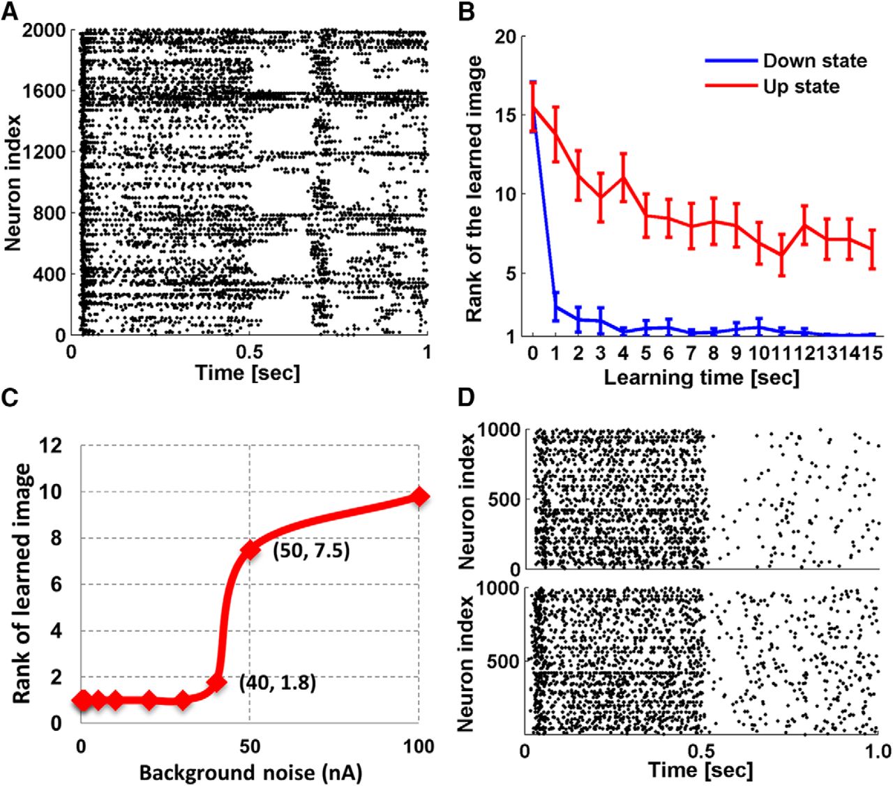
Legenstein and Maass also identified the existence of up and down-states (Cowan and Wilson, 1994) in their simulated neural network models. These states refer to dynamic regimes observed in intracellular recordings of mammalian central nervous system neurons that differ in their membrane potential and conductance properties. In the down-states, the membrane potential is hyperpolarized and stable and membrane conductance is low. In the up-states, the membrane potential is more depolarized, highly variable and membrane conductance is high, resulting from a continuous bombardment of background synaptic inputs. In neural networks, up-states are characterized by network-wide synchronized bursting activity (Johnson and Buonomano, 2007). As no bursting was observed in our simulations, it seems that the tuned Wscale and λ parameters constrained the networks to be in down-states. To know how bursting would affect the network performance, we removed the biological boundaries of the parameters. In one simulation, we increased Wscale tenfold while preserving λ. Bursting emerged during stimulus presentations (Fig. 9A), and we measured network accuracy through single face recognition simulations and compared the results with the results described above (Fig. 9B). It turns out that in a bursting network, network performance is compromised, and more learning is required for comparable accuracy. Bursting also emerged with a twofold increase in λ while preserving Wscale, which induced similar impairments of network accuracy.

Effect of bursting and noise. A, Response of a 20 × 20 × 5 up-state network after learning a human face image for 11 s. A network burst spontaneously emerged in the interval of 0.5–1.0 s when no input stimulus was given. B, Impact of bursting on network performance. Rank of network firing rate to the familiar image among 30 testing images is plotted as a function of learning time. Blue represents simulations with down-state networks, the same networks as we used in the single face recognition simulations. Red represents simulations with up-state networks (Wscale was set tenfold of the original value used in simulation). Error bars are the SEM of 90 simulations conducted on 30 networks. C, Impact of background noise on network performance. Average rank of network firing rate to the familiar image among 30 test images after learning for 15 s is plotted as a function of background noise. D, Network spiking activity of a 20 × 20 × 5 network to the input stimulus, simulated with 40- and 50-nA background noise, respectively.
Network accuracy is also affected by the amount of background noise current injected into the neurons (Eq. 1) during simulation. We measured network accuracy through single face recognition simulations with background noise ranging from 1 to 100 nA. Figure 9C shows that network accuracy is preserved until the noise exceeds 40 nA, which is unrealistically high compared with normal ranges used in CSIM. A dramatic performance decline is seen from 40 to 50 nA, and the corresponding network responses are exemplified in Figure 9D. Background noise of 50 nA clearly introduced more random spikes during simulation. If the number of random spikes exceeds the discrepancy of firing rate that was previously used to differentiate familiarity from novelty, it is very likely to disrupt network performance.
Discussion
In the simulations described above, we have investigated the ability of recurrent spiking neural networks supplemented with NMDAR plasticity to detect familiar sensory inputs following unsupervised learning. Unsupervised learning is biologically plausible and has been shown to be critical for the development of the mammalian central nervous system, for example, in the visual pathway (Blasdel et al., 1977). In the beard versus no-beard classification simulations, our neural networks learned to differentiate “beard” and “no-beard” face images. The single face recognition simulations were conducted with a more rigorous design to investigate the specificity of familiarity detection. Networks of 20 × 20 × 5 neurons connected by NMDAR-containing synapses were able to detect a previously-seen face accurately in most of the simulations, with a pronounced and specific increase in overall firing rate for the familiar stimulus. Responses to the control groups did not deviate far from baseline.
Our simulations with larger networks (up to 50 × 50 × 6 neurons) indicated that multiple familiarity traces can be learned and stored. The storage capacity increased with available network space. Our largest network model (15,000 neurons) can store familiarity traces for 60 faces, before accuracy drops to chance level. One possible explanation is that within large networks, subsets of synaptic connections that are selectively potentiated or depressed for each face can co-exist, reducing the chance of a new memory overwriting an older one. This observation suggests a potential resolution for the stability-plasticity dilemma. Considering there are billions of neurons in the human brain organized in a very large number of microcircuits, it seems reasonable, in principal, that human recognition memory has an apparently limitless capacity, as reported by Standing’s experiments (1973). Nevertheless, it is important to mention that in Standing’s tests, a two-alternative forced-choice paradigm was used. In a subsequent study that supported Standing’s finding on memory capacity (Brady et al., 2008), the two-choice paradigm was also used. A higher rate of recall error was reported by Laeng et al. (2007), when conducting similar image recognition experiments using a yes-no paradigm with only one picture presented. Whether the two-choice paradigm is justified as a good measure for recognition and a good indication for memory capacity is arguable (Laeng et al., 2007). Our analysis relied on a comparative paradigm similar to Standing’s two-alternative tests: to interpret the data and measure familiarity, a threshold needs to be set for the network firing rate, which was done empirically comparing familiar and novel responses. Once the threshold is set, the networks can also make yes-no decisions for individual inputs (Fig. 4G).
In addition to the specificity and capacity for familiarity detection, we also noticed a generalization effect in the responses of the trained networks to input stimuli. Evidence for generalization was observed when, following training, the response to novel input stimuli was increased selectively for those that belonged to the same class as the trained inputs. In the beard versus no-beard classification simulations, generalization was observed when the trained networks were able to distinguish novel beard from novel no-beard images. In single face recognition simulations, the networks generalized familiarity response to a subset of images from the same class as the presented stimulus. In the multi-face recognition simulations, the networks apparently learned the concept face after training on ten face images: they responded stronger to novel faces than their scrambled versions. Recall that for 10 × 10 × 5 networks, input neurons were set to form synapses one-to-one with the first layer of the network reservoir, whereas for networks of 20 × 20 × 5 or larger dimension, input neurons were set to form synapses randomly with the network reservoir by probability. Innervation by probability is a better way to use the network space and prevents overtraining of the first layer of the network reservoir. Meanwhile it disrupts the spatial patterns present in the face images, making the familiarity detection a high-dimensional challenge. Yet the generalization property remained with the randomly projected inputs, which speaks to the robustness and computational power of our networks, i.e., learning specificity was preserved while generalization was acquired. When multiple inputs from a class were learned, generalization allowed the networks to act as an unsupervised classifier, by automatically classifying input stimuli based on past sensory experience. In contrast, conventional classifiers require properly labeled data of all classes to be trained.
Fisher’s discriminant analyses suggest that familiarization occurred in high-dimensional feature space. Network connections were modified and neurons in hidden circuits were recruited to respond to familiar inputs. Neurons hidden from the input layer are analogous to neurons from deep layers of a feed-forward network, or neurons from the downstream circuits in higher-order brain regions. Their recruitment suggests how signals can be relayed to brain regions other than the primary processing region and cause differences in neuronal activity. As the deep-layer neurons showed unique firing patterns to the familiar stimulus, their activity can be used to identify the input pattern, a function similar to the “grandmother-cells” identified by in vivo brain recordings (Quiroga et al., 2005). For decades neuroscientists have debated the possible forms of information encoding in the brain, such as parallel distributed processing versus single neuron firing. Results presented here show they are not mutually exclusive. While a familiar input is encoded in a network of thousands of neurons, it may also selectively activate single neurons in deep layers.
Familiarity studies stemmed from experiments at the behavioral level. Several groups have conducted experiments with the familiarity/novelty paradigm in vivo. Studies using fMRI measurements (Kosaka et al., 2003; Gobbini and Haxby, 2006) found an increase in the BOLD signal to familiar stimuli. Recordings in the inferior temporal lobe of behaving monkeys have demonstrated differential responses to novel and familiar images (Anderson et al., 2008). Interestingly, familiar images evoked larger-amplitude local field potentials, whereas multi-unit spiking responses were greater for novel images. Finally, a phenomenon called stimulus-selective response potentiation was identified in rodent visual cortex recordings (Frenkel et al., 2006; Cooke and Bear, 2010; Gavornik and Bear, 2014). It is a form of experience-dependent response enhancement during visual experiments. We think it supports the existence of intrinsic familiarity in the visual cortex.
A few neural network models have been proposed to study network-level learning and memory. Several of them applied STDP to various network architectures. For example, a few groups (Lazar et al., 2007; Oliveri et al., 2007; Xue et al., 2013) investigated LSMs with STDP and the results suggested an enhanced computational capability. In these models, STDP was either applied to train readout neurons or to modulate neuron excitability, rather than allowing it to directly modify synaptic weights in the network. Studies that used neural networks other than LSMs (Clopath et al., 2010; Carlson et al., 2013; Klampfl and Maass, 2013; Zheng et al., 2013; Srinivasa and Cho, 2014) have reported emerging learning and memory after applying STDP to recurrent network architectures. Nevertheless, the networks they used are either of a preimposed wiring diagram (Klampfl and Maass, 2013) or highly simplified (Srinivasa and Cho, 2014), and therefore poorly replicate cortical microcircuits. Furthermore, these studies solely consider STDP for plasticity while we combine the two major forms of plasticity, LTD/LTP (frequency rule) and STDP (timing rule), based on the calcium control hypothesis, rather than phenomenological equations. Evidence for the interplay of LTD/LTP and STDP has been found in the literature, and separating them by firing rate or spike timing might lead to an artificial dichotomy (Sjöström et al., 2001). Our simulation results suggest a mutual-enhancing effect by combining STDP with LTP/LTD, and this could potentially explain one-shot familiarity memory (Yakovlev et al., 2008). Additionally, some of the reported models require homeostatic control (Clopath et al., 2010; Carlson et al., 2013; Zheng et al., 2013) or inhibitory-STDP (Srinivasa and Cho, 2014) to attain network stability, but in our NMDAR-LSM networks, we relied on the intrinsic balance between LTD and LTP instantiated by the calcium control hypothesis for stability.
The plasticity model we implemented was created to model bidirectional synaptic plasticity through NMDARs (Shouval et al., 2002). Whether NMDARs are solely responsible for this form of plasticity is still controversial, as voltage-dependent Ca2+ channels (Nevian and Sakmann, 2006) and metabotropic glutamate receptors (Gladding et al., 2009) have been reported to be capable of inducing synaptic plasticity as well. Yet there is growing evidence that bidirectional modifications can be induced through NMDAR-dependent pathways alone (Hunt et al., 2013; Huang et al., 2014). The results presented here demonstrate that bidirectional synaptic plasticity is sufficient to endow neural network models of generic cortical microcircuits with the ability to detect familiar sensory inputs through unsupervised learning. This has important consequences for mammalian brain development, since it suggests that these universal building blocks of the cortex have an inherent ability for familiarity detection.
In NMDAR-LSM networks, recurrent spiking neural networks expand input stimuli into high-dimensional feature space (Maass et al., 2002). Unsupervised learning altered the feature space to allow linear separation of familiar from novel faces, by formation of subnetworks specific for each input stimulus. Learning multiple inputs belonging to a class (e.g., beard, face) resulted in generalization, allowing the network to classify novel input stimuli. This relationship between familiarity detection, generalization, and classification needs to be studied in more depth.
Note Added in Proof: The title of the article was incorrectly listed in the Early Release version. The title has now been corrected.
Footnotes
The authors declare no competing financial interests.
This work was supported by grants MOE2012-T2-1-039 from the Singapore Ministry of Education and OFIRG/0019/2016 from the National Medical Research Council (to A.M.J.V.) and by an award from the Singapore Ministry of Health and A*STAR, the Agency for Science, Technology and Research.
This is an open-access article distributed under the terms of the Creative Commons Attribution 4.0 International license, which permits unrestricted use, distribution and reproduction in any medium provided that the original work is properly attributed.
References
In this issue


