

Article Figures & Data
Figures
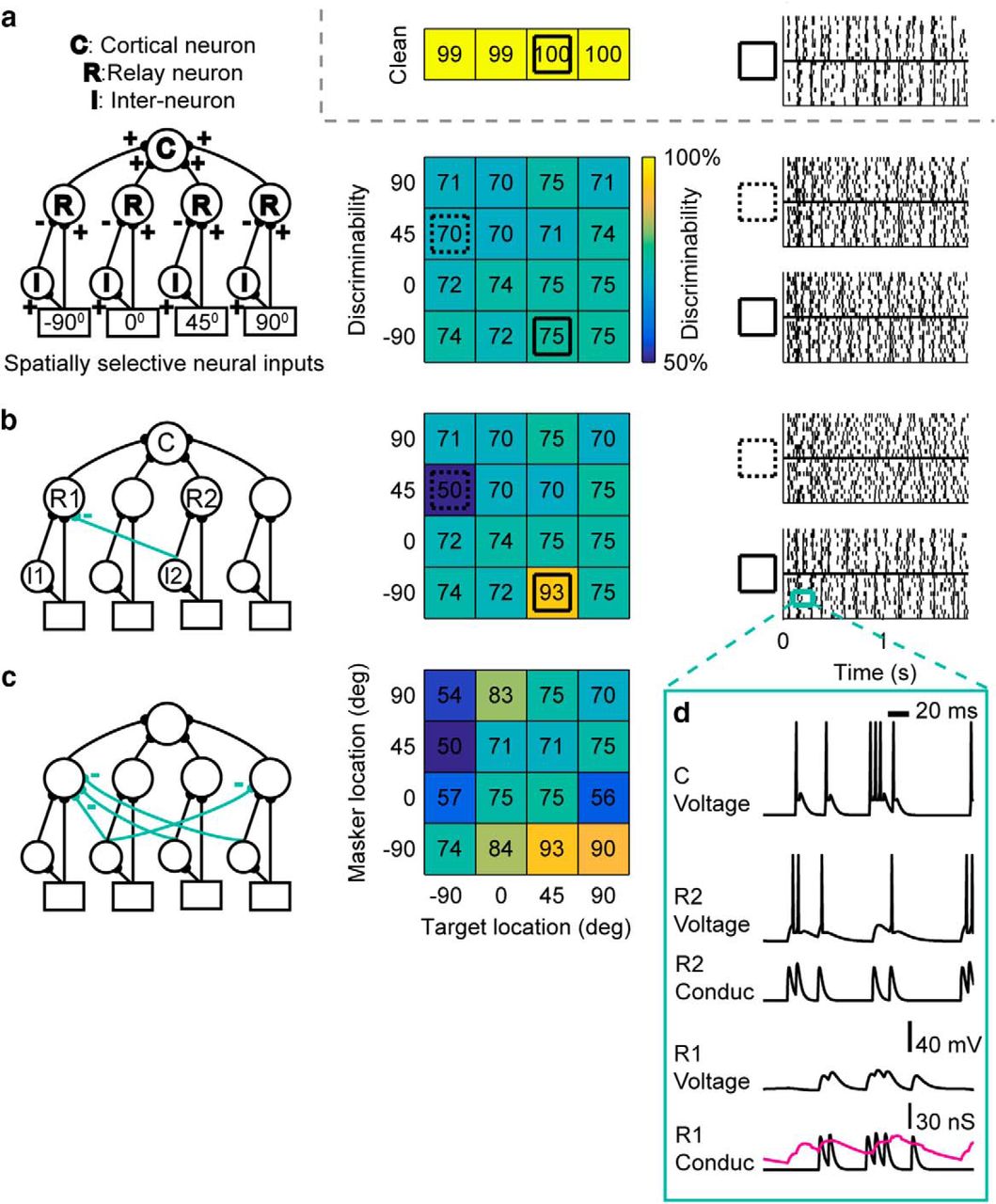
- Figure 1.
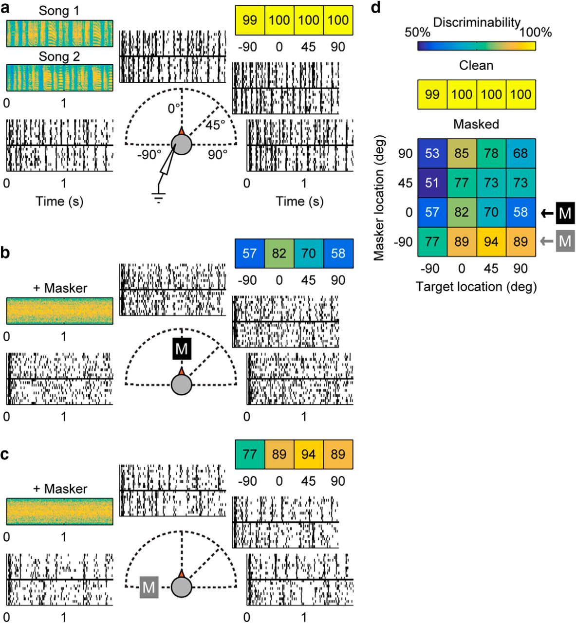
Recorded cortical neurons develop sharper spatial responses to targets when a noise masker is present (Maddox et al., 2012). a, Responses to target alone. Two bird songs—Song 1 and 2 (spectrograms shown in top left)—are played separately from four locations −90°, 0°, 45°, and 90°. Recorded raster plots of responses to the two birdsongs are shown at each azimuth location. Positive degrees indicate locations contralateral to recording site. The color-coded discriminability values for each location are shown in the horizontal grid on the upper right. (Color map for all panels is shown in d, top row.) b, c, Responses to target with masker. Masker and one target song are played concurrently from one (colocated) or two (separated) of the four stimulus locations. A masker fixed at 0° or −90°, indicated by a black or grey boxed M, respectively, whereas the target song is played at one of the locations shown. As in a, recorded raster responses from each target location are shown, and discriminability values are shown in the colored grid of values (top right). d, Discriminability values for all location combinations. The top grid (single row) of numbers are the discriminability values for the “clean” (target-alone) conditions. In the lower, spatial discriminability grid, each block indicates a target and masker location combination. The rows indicated by a black or grey boxed M are cases where the masker is fixed at 0° or −90°. Blocks in all grids are colored according to the color scale given at the top of this panel.
- Figure 2.
Lateral inhibition in the model can account for the spatial tuning and spatial segregation properties of recorded units. a–c, Left, Model structure. Center, Simulated spatial grid. Right, Raster plots for stimulus conditions indicated by dashed or solid squares in the grid. Top right, Inset, The simulated discriminability for the clean (no-masker) case indicating broad spatial tuning. This clean case is not impacted by the addition of lateral inhibition, and is identical for all networks shown. a, Basic model structure with no lateral inhibitory connections. Simulated multisource spatial grid in model without lateral inhibition lacks the spatial diversity observed in the data. b, Spatial grid produced by the model with one inhibitory connection between 0° and −90°, shows an increase in discriminability when target and masker are presented at 0° and −90°, respectively. c, Model with additional inhibitory connections simulates the spatial response of the recorded unit shown in Figure 1d. d, Subthreshold responses of relay and cortical neurons, R1, R2, and C (b, left), for the labeled time segment (b, right) of one trial when target is presented at 0° and masker at −90°. Direct excitatory currents to R1 (R1 Conduc: black curve) are offset by inhibitory currents from I2 (R1 Conduc: magenta curve), and R1 is unable to reach spiking threshold, as seen in its voltage trace (R1 Voltage: black curve). In contrast, R2 is able to relay its temporal information to C, whose spiking pattern (C Voltage) resembles that of R2 (R2 Voltage).
- Figure 3.
Illustration of model input generation process. The stimulus spectrogram was convolved with STRFs modeled after midbrain neurons, followed by half-wave rectification, then rate normalization to generate an instantaneous output-firing rate. This firing rate was then used to generate spikes using a spiking model (see Materials and Methods for details). The values of temporal phase Pt and normalization factor a used were reported in Table 2.
- Figure 4.
Network performance is robust to broader spatial tuning of inputs, as shown by extended simulations on the example unit previously displayed in Figure 2. a, Illustrations of Gaussian spatial tuning curves of varying widths, defined by twice the standard deviation (2σ). b, Results of spatial grid simulations for broadened input tuning width 2σ at 40°, 80°, and 120°, compared with the no-overlap case (<15°) on the bottom. The cross-correlation coefficient and deviation of the simulated results are plotted in green and purple, respectively, on separate horizontal axes. On the cross-correlation coefficient axis (top), larger values (closer to unity) indicate a better fit, whereas the deviation axis (bottom) shows better fits at smaller values closer to 0%. For reference, shaded areas and dotted lines indicate the mean and standard deviation of cross-correlation coefficient and deviation values, for original simulated population using non-overlapping inputs. As the spatial tuning of input units was broadened from <15° to 120°, the correlation coefficient (green dots) and the deviation (purple dots) degraded gracefully. The correlation coefficient remained above 0.8 and the deviation remained below 10% for the broadest tuning width. c, Illustrations of simulated spatial grids with input widths of 40° and 120°. The 40° spatial grid can be compared with the no overlap spatial grid shown in Figure 2c . The two grids show a similar visual pattern, which is quantified by the similar deviation and cross-correlation coefficient values shown in b. The 120° grid maintains the general pattern but has overall higher discriminability throughout.
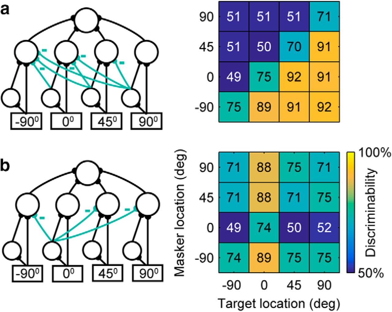
- Figure 5.
Engineering solutions. a, Left, “Contralateral-dominance” model network where all channels contralateral to the dominant channel are inhibited. Right, Simulation results of this structure achieve the maximum number of spatially separable target and masker locations, where all targets contralateral to masker can be segregated. b, Left, “Beamformer” model network where the channel tuned to the front (0°) inhibits all other channels. Right, The simulated spatial grid illustrating the segregation of the frontal target source.


Tables
STRF no. Neural units Adaptation conductance 1 3, 6, 9, 10, 11, 13, 21, 23 0.025 14, 22 0.04 2 15 0 3 29 0.12 27 0.1 4 7 0.07 5 19 0.06 6 2 0.06 7 5 0.2 25 0.16 8 20, 32 0.07 1, 12, 33 0.08 9 16, 23 0.09 10 8 0.09 11 4 0.09 12 26, 28, 31 0.03 13 17 0.01 18 0.03 STRF input and adaptation conductance were fit to best match the firing characteristics of each neuron recorded in the Maddox et al. (2012) study, whereas other neuron modeling parameters were fixed as reported above.
STRF no. Normalization factor  (rad)
(rad)1 0.08 1.4608 2 0.1 1.4923 3 0.07 1.508 4 0.1 5 0.12 1.5237 6 0.1 1.5394 7 0.07 1.5425 8 0.087 9 0.15 1.5582 10 0.05 11 0.08 12 0.16 1.5598 13 0.17 1.5708 Temporal phase
and normalization factor are adjusted to match the recorded responses of the corresponding neurons, while other temporal and spectral parameters are held fixed and reported above.


In this issue


Jump to section
- Article
- Visual Abstract
- Abstract
- Significance Statement
- Introduction
- Methods
- Quantifying goodness of fit
- Results
- Cross-channel lateral inhibition enables the network to match experimentally observed neural responses
- Spatial tuning
- Extending the model network to potential engineering solutions for segregating spatial sound sources
- Discussion
- Predictions and implications
- Footnotes
- References
- Synthesis
- Figures & Data
- Info & Metrics
- eLetters