1
Laboratoire Psychologie de la Perception, Centre National de la Recherche Scientifique and Université Paris Descartes, Paris, France
2
Département d’Etudes Cognitives, Ecole Normale Supérieure, Paris, France
Spiking models can accurately predict the spike trains produced by cortical neurons in response to somatically injected currents. Since the specific characteristics of the model depend on the neuron, a computational method is required to fit models to electrophysiological recordings. The fitting procedure can be very time consuming both in terms of computer simulations and in terms of code writing. We present algorithms to fit spiking models to electrophysiological data (time-varying input and spike trains) that can run in parallel on graphics processing units (GPUs). The model fitting library is interfaced with Brian, a neural network simulator in Python. If a GPU is present it uses just-in-time compilation to translate model equations into optimized code. Arbitrary models can then be defined at script level and run on the graphics card. This tool can be used to obtain empirically validated spiking models of neurons in various systems. We demonstrate its use on public data from the INCF Quantitative Single-Neuron Modeling 2009 competition by comparing the performance of a number of neuron spiking models.
Neurons encode time-varying signals into trains of precisely timed spikes (Mainen and Sejnowski, 1995
; Brette and Guigon, 2003
), using a diverse set of ionic channels with specific characteristics. Recently, it was found that simple phenomenological spiking models, such as integrate-and-fire models with adaptation, can in fact predict the response of cortical neurons to somatically injected currents with surprising accuracy in spike timing (Jolivet et al., 2004
; Brette and Gerstner, 2005
; Gerstner and Naud, 2009
). This unexpected performance is probably related to the fact that detailed conductance-based models with widely diverse ion channel characteristics can in fact have the same properties at neuron level (Goldman et al., 2001
). These encouraging results triggered an interest in quantitative fitting of neuron models to experimental recordings, as assessed by the recent INCF Quantitative Single-Neuron Modeling competition. The competition has seen several successful submissions, but there is no available method to systematically fit arbitrary models to experimental data. Such computational tools would be particularly useful for modellers in systems neuroscience, for example, who could use empirically validated models in their studies. We developed a model fitting library, which works with the Brian simulator (Goodman and Brette, 2009
), and allows the fitting of user-defined spiking models to electrophysiological data consisting of spike trains elicited by time-varying signals (for example, intracellularly injected currents). If the user’s machine has a graphics processing unit (GPU) − a cheap parallel processor available on many standard machines − the algorithms run in parallel on it. The library is available as a part of Brian, which is distributed under a free open-source license
1
.
There are several important difficulties in this model fitting problem. Firstly, because of the threshold property, the mapping from a time-varying signal to spike trains is generally discontinuous in spiking models (Brette, 2004
). Besides, the fitness criterion we used (the gamma coincidence factor used in the INCF competition; Jolivet et al., 2008
) is discrete, because it is a function of the number of coincidences within a predefined temporal window. These facts prevent us from using optimization methods based on gradients (e.g. conjugated gradient descent). Secondly, a single evaluation of the criterion for a given set of parameter values involves the simulation of a neuron model over a very long time. For example, recordings in challenges A and B of the 2009 INCF competition last 60 s, sampled at 10 kHz, totalling 600,000 values of the input signal. Thus, evaluating the fitness criterion for any spiking model involves several millions of operations. Thirdly, not only the parameter values are unknown, but there are also many candidate models. In particular, it is not unreasonable to think that different neuron types may be best fit by different phenomenological models. Therefore, the optimization tools should be flexible enough to allow testing different models.
To address these issues, we developed a model fitting toolbox for the spiking neural network Brian (Goodman and Brette, 2009
). Brian is a simulator written in Python that lets the user define a model by directly providing its equations in mathematical form (including threshold condition and reset operations). Using an interpreted language such as Python comes at a cost, because the interpretation overhead can slow down the simulations, but this problem can be solved by vectorizing all operations when the network model includes many neurons. It turns out that the same strategy applies to programming GPUs, which are most efficient when all processors execute the same operation (the Single Instruction, Multiple Data (SIMD) model of parallel programming). Therefore, we developed several vectorization techniques for spiking model optimization (see Vectorization Techniques). These techniques apply both to CPU simulations and to parallel GPU simulations. We used just-in-time compilation techniques to keep the same level of flexibility when models are simulated on the GPU, so that using the GPU is transparent to the user (see GPU Implementation). We demonstrate our algorithms (see Results) by fitting various spiking models to the INCF competition data (challenges A and B). Consistent with previous studies, we found that adaptive spiking models performed very well. We also show how our tool may be used to reduce complex conductance-based models to simpler phenomenological spiking models.
Vectorization Techniques
Fitting a spiking neuron model to electrophysiological data is performed by maximizing a fitness function measuring the adequacy of the model to the data. We used the gamma factor (Jolivet et al., 2008
), which is based on the number of coincidences between the model spikes and the experimentally-recorded spikes, defined as the number of spikes in the experimental train such that there is at least one spike in the model train within ±δ, where δ is the size of the temporal window (typically a few milliseconds). The gamma factor is defined by
where Ncoinc is the number of coincidences, Nexp and Nmodel are the number of spikes in the experimental and model spike trains, respectively, and rexp is the average firing rate of the experimental train. The term 2δNexprexp is the expected number of coincidences with a Poisson process with the same rate as the experimental spike train, so that Γ = 0 means that the model performs no better than chance. The normalization factor is chosen such that Γ ≤ 1, and Γ = 1 corresponds to a perfect match. The gamma factor depends on the temporal window size parameter δ (it increases with it). However, we observed empirically that the parameter values resulting from the fitting procedure did not seem to depend critically on the choice of δ, as long as it is not so small as to yield very few coincidences. For most results shown in the Section “Results”, we chose δ = 4 ms as in the INCF competition.
This fitting problem can be solved with any global optimization algorithm that does not directly use gradient information. These algorithms are usually computationally intensive, because the fitness function has to be evaluated on a very large number of parameter values. We implemented several vectorization techniques in order to make the fitting procedure feasible in a reasonable amount of time. Vectorization allows us to use the Brian simulator with maximum efficiency (it relies on vectorization to minimize the interpretation overhead) and to run the optimization algorithm in parallel.
Vectorization over parameters
Particle swarm optimization algorithm. We chose the particle swarm optimization (PSO) algorithm (Kennedy and Eberhart, 1995
), which involves defining a set of particles (corresponding to parameter values) and letting them evolve in parameter space towards optimal values (see Figures 1 and 7
). Evaluating the fitness of a particle requires us to simulate a spiking neuron model with a given set of parameter values and to calculate the gamma factor. Since the simulations are independent within one iteration, they can be run simultaneously. In the PSO algorithm, each particle accelerates towards a mixture of the location of the best particle and the best previous location of that particle. The state update rule combines deterministic and stochastic terms in order to prevent the particles from getting stuck in locally optimal positions:
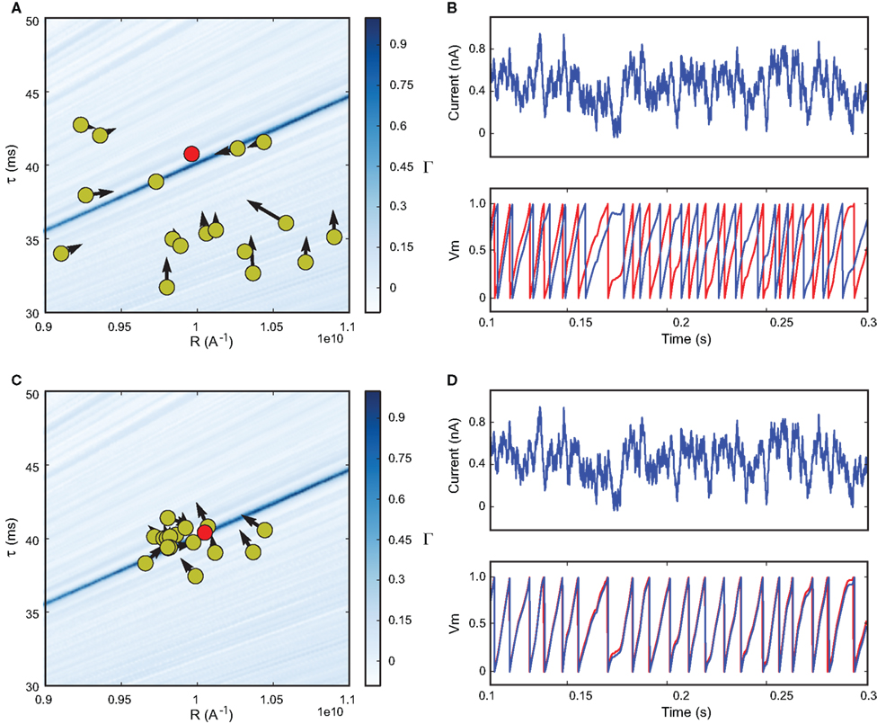
Figure 1. Fitting spiking neuron models with particle swarm optimization (PSO). The target spike train was generated by injecting a noisy current (white noise, 500 ms long) into a leaky integrate-and-fire model (R = 1010 A−1 and τ = 40 ms), and PSO was run to find the correct parameter values. The boundary conditions used for the optimization are the ranges of the axes. The optimization algorithm makes the particles (sets of parameter values) evolve towards the area with high fitness values (an oblique line in this example). (A) Positions of the particles in parameter space (R, τ) at the start of the algorithm and their evolution at the next iteration (arrows). The colored background represents the value of the gamma factor for all parameter values. (B) Voltage trace of the red particle shown in A compared to the original one (blue), in response to the injected current (top). The y-axis is unitless. (C) Positions of the particles at iteration 4. (D) Voltage trace of the red particle (same as in (A) and (B)) at iteration 4. The gamma factor increased from 0.09 to 0.55 between (B) and (D).
where Xi(t) and Vi(t) are the position and speed vectors of particle i at time t, respectively.  is the best position occupied by particle i before time t (local best position), and Xg(t) is the best position occupied by any particle before time t (global best position). ω, cl and cg are three positive constants which are commonly chosen as follows in the literature (Shi and Eberhart, 1998
; den Bergh, 2006
): ω = 0.9, cl = cg = 1.9. We chose these values for most results shown in this paper. For the in vitro recordings, we chose cl = 0.1 and cg = 1.5 which we empirically found to be more efficient. Finally, rl and rg are two independent random numbers uniformly resampled between 0.0 and 1.0 at each iteration.
is the best position occupied by particle i before time t (local best position), and Xg(t) is the best position occupied by any particle before time t (global best position). ω, cl and cg are three positive constants which are commonly chosen as follows in the literature (Shi and Eberhart, 1998
; den Bergh, 2006
): ω = 0.9, cl = cg = 1.9. We chose these values for most results shown in this paper. For the in vitro recordings, we chose cl = 0.1 and cg = 1.5 which we empirically found to be more efficient. Finally, rl and rg are two independent random numbers uniformly resampled between 0.0 and 1.0 at each iteration.Boundary constraints can be specified by the user so that the particles are forced to stay within physiologically plausible values (e.g. positive time constants). The initial values Vi(0) are set at 0, whereas the initial positions of the particles are uniformly sampled within user-specified parameter intervals. The convergence rate of the optimization algorithm decreases when the interval sizes increase, but this effect is less important when the number of particles is very large.
Fitness function. The computation of the gamma factor can be performed in an offline or online fashion. The offline method consists in recording the whole spike trains and counting the number of coincidences at the end of the simulation. Since the fitness function is evaluated simultaneously on a very large number of neurons, this method can be both memory-consuming (a large number of spike trains must be recorded) and time-consuming (the offline computation of the gamma factor of the model spike trains − which can consist of several hundred thousand spikes − against their corresponding target trains is performed in series). The online method consists in counting coincidences as the simulation runs. It allows us to avoid recording all the spikes, and is much faster than the offline algorithm. Moreover, on the GPU the online algorithm requires a GPU to CPU data transfer of only O(num particles) bytes rather than O(num spikes), and CPU/GPU data transfers are a major bottleneck. Our fitting library implements the online algorithm. About 10% of the simulation time at each iteration is spent counting coincidences with our algorithm on the CPU.
Vectorization over data sets
The particle swarm algorithm can be easily adapted so that a single neuron model can be fitted to several target spike trains simultaneously. The algorithm returns as many parameter sets as target spike trains. The gamma factor values for all particles and all spike trains are also computed in a single run, which is much faster than computing the gamma factors in series. For example, in the INCF Quantitative Modeling dataset, all trials (13 in challenge A and 9 in challenge B) can be simultaneously optimized.
Vectorization over time
The gamma factor is computed by simulating the neurons over the duration of the electrophysiological recordings. The recordings can be as long as several tens of seconds, so this may be a bottleneck for long recordings. We propose vectorizing the simulations over time by dividing the recording into equally long slices and simulating each neuron simultaneously in all time slices. Spike coincidences are counted independently over time slices, then added up at the end of the simulation when computing the gamma factor. The problem with this technique is that the initial value of the model at the start of a slice is unknown, except for the first slice, because it depends on the previous stimulation. To solve this problem, we allow the time windows to overlap by a few hundreds of milliseconds and we discard the initial segment in each slice (except the first one). The initial value in the initial segment is set at the rest value. Because spike timing is reliable in spiking models with fluctuating inputs (Brette and Guigon, 2003
), as in cortical neurons in vitro (Mainen and Sejnowski, 1995
), spike trains are correct after the initial window, that is, they match the spike trains obtained by simulating the model in a single pass, as shown in Figure 2
.
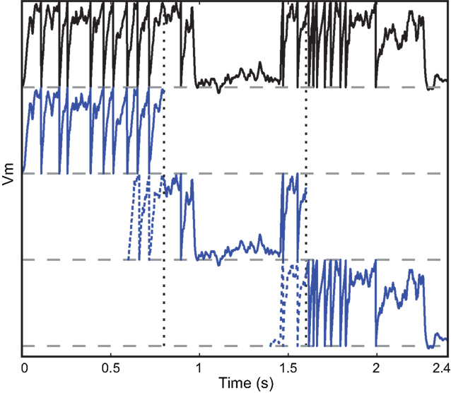
Figure 2. Vectorization over time. A leaky integrate-and fire neuron receiving a dynamic input current is simulated over 2.4 s (top row, black). The same model is simultaneously simulated in three time slices (blue) with overlapping windows (dashed lines). Vertical dotted lines show the slice boundaries. The model is normalized so that threshold is 1 and reset is 0. The overlap is used to solve the problem of choosing the initial condition and is discarded when the slices are merged.
The duration of one slice is overlap + recording duration/number of slices, so that the extra simulation time is overlap × number of slices, which is, relative to the total simulation time, overlap/slice duration. Thus, there is a trade off between the overhead of simulating overlapping windows and the gain due to vectorisation. In our simulations, we used slices that were a few seconds long. The duration of the required overlap is related to the largest time constant in the model.
GPU Implementation
A graphics processing unit (GPU) is a type of chip available on modern graphics cards. These are inexpensive units designed originally and primarily for computer games, which are increasingly being used for non-graphical parallel computing (Owens et al., 2007
). The chips contain multiple processor cores (240 in the current state of the art designs, and 512 in the next generation which will be available in 2010) with a limited ability to communicate between each other. This makes them ideal for the particle swarm algorithm where many independent simulations need to be run for each iteration of the algorithm, especially with the vectorization techniques that we presented in the Section “Vectorization Techniques”.
Programming for a GPU is rather specialised. Each processor core on a GPU is much simpler than a typical CPU, and this places considerable limitations on what programs can be written for them. Moreover, although recent versions of these chips allow more of the functionality of a full CPU (such as conditional branching), algorithms that do not take into account the architecture of the GPU will not use it efficiently. In particular, the GPU places constraints on memory access patterns. Consequently, although 240 cores may be present in the GPU, it is unrealistic in most cases to expect a 240× speed increase over a CPU. However, speed improvements of tens to hundreds of times are often possible (see the showcase on the NVIDIA CUDA Zone)
2
. In our case, we have achieved a roughly 50−80× speed improvement, thanks largely to the fact that the model fitting algorithm is “embarassingly parallel”, that is, that it features a number of independent processes which do not interact with each other. This means that memory can be allocated in the topologically continuous fashion that is optimal for the GPU, and the code does not need to introduce synchronization points between the processes which would slow it down.
We use the GPU in the following way. We have a template program written in the subset of C++ that runs on the GPU. Code that is specific to the neuron model is generated and inserted into the template when the model fitting program is launched. The code is generated automatically from the differential equations defining the neuron model, compiled and run automatically on the GPU (just-in-time compilation) using the PyCUDA package (Klöckner et al., 2009
).
The code generation works as follows. We start from a basic template that handles standard operations shared amongst all models, including loading the input currents to the model, computing the coincidence count and so forth. The template has several slots for specifying code specific to the model, including the numerical integration step and the thresholding and reset behavior. The differential equations defining the neuron model are stored as strings in Brian. For example, if the differential equation was
'dV/dt=-V/tau' then we store the substring '-V/tau'. An Euler solver template for this might look like:
In the case above this would become (after substitutions):
This latter code snippet is valid C code that can be run on the GPU. A similar technique is used for thresholding and reset behaviour.
These techniques mean that the huge speed improvements of the GPU are available to users without them having to know anything about GPU architectures and programming. Usage is transparent: on a system with a GPU present and the PyCUDA package installed, the model fitting code will automatically be run on the GPU, otherwise it will run on the CPU.
Distributed Computing
As mentioned in the previous section, the model fitting algorithm presented here is close to “embarassingly parallel”, meaning that it can relatively easily be distributed across multiple processors or computers. In fact, the algorithm consists of multiple iterations, each of which is “embarassingly parallel” followed by a very simple computation which is not. More precisely, the simulation of the neuron model, the computation of the coincidence count, and most of the particle swarm algorithm can be distributed across several processors without needing communication between them. The only information that needs to be communicated across processors is the set of best parameters found so far. With N particles and M processors, each processor can independently work on N/M particles, communicating its own best set of parameters to all the other processors only at the end of each iteration. This minimal exchange of information means that the work can be efficiently distributed across several processors in a single machine, or across multiple machines connected over a local network or even over the internet. We use the standard Python multiprocessing package to achieve this. See the section titled “Benchmark” and Figure 6
for details on performance.
Model Fitting
We checked our algorithms on synthetic data and applied them to intracellular in vitro recordings.
Synthetic data
We first check that the optimization algorithms can fit a spiking neuron model to spike trains generated by the same model (Figure 3
). We simulated a leaky integrate-and-fire neuron model with an adaptive threshold (equations in Table 1
) responding to a fluctuating current injection over 500 ms (Ornstein-Uhlenbeck process). As expected, the optimization algorithm converged to a perfect fit (Γ = 1 with precision δ = 0.1 ms) after just a few iterations. We chose this small value of δ to show that the fit can be nearly perfect, as expected in this situation. The corresponding parameter values were very close to the original ones (±15%), so that the original and optimized traces match, even though only the spike trains were used for the fitting procedure (a perfect match of the traces can be obtained by using more particles than we used for the figure, giving parameters values within ±3%). However, this is not likely to be a general result: for example, if the neuron model included after-spike effects (such as refractoriness) and the interspike intervals were longer than these effects (that is, at low firing rates), then the method could not recover these properties since they would not be visible in the spike trains.
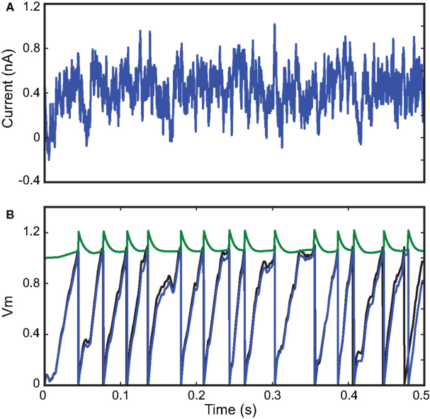
Figure 3. Fitting a leaky integrate-and-fire model with adaptive threshold. (A) A 500-ms fluctuating current is injected into a leaky integrate-and-fire neuron with adaptive threshold (R = 3.4 × 10⁹ A−1, τ = 25 ms, τt = 10 ms, α = 0.15, a = 0.1). The output spike train is used as the target spike train for the fitting procedure with the same model. (B) Results from the optimization algorithm match the original parameters within 15% error and the resulting trace (blue; threshold in green; the model is normalized so that Vm has no unit) is close to the original trace (black), even though only spike timings were used for fitting. The gamma factor was 1.0 at precision δ = 0.1 ms.
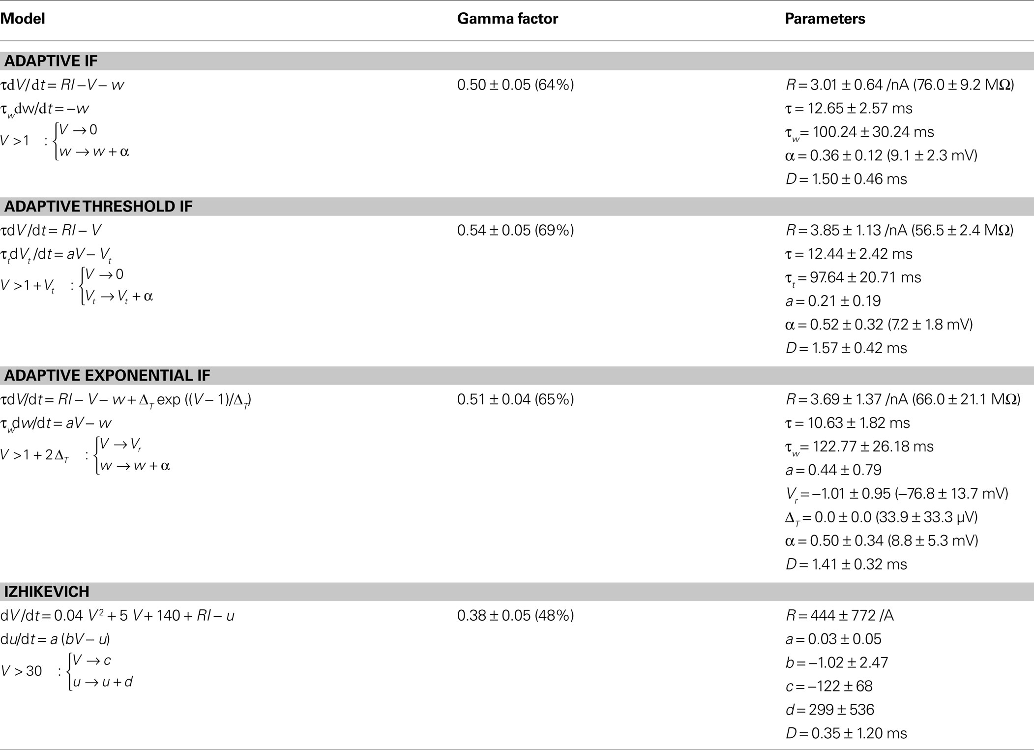
Table 1. Optimization results for Challenge A. Four neuron models were fitted to the electrophysiological recordings of a regular spiking L5 pyramidal cell responding to in-vivo-like current injection. There were 13 trials with the same input. The models were optimized on the part of the data between 17.5 seconds and 28 seconds and the gamma factors were calculated between 28 and 38 seconds (δ = 4 ms). The value relative to the intrinsic reliability Γin is reported in brackets. Parameter D is a time shift for output spikes (recorded spikes typically occur slightly after model spikes because they are reported at the time when the membrane potential crosses 0 mV). We also reported rescaled versions of the parameter values (in brackets) so that they correspond to electrophysiological quantities.
In vitro recordings
We then applied our fitting procedure to in vitro intracellular recordings from the 2009 Quantitative Single-Neuron Modeling competition (challenges A and B). In these recordings, fluctuating currents were injected into the soma of cortical neurons (L5 regular spiking pyramidal cell for challenge A and L5 fast spiking cell for challenge B). Figure 4
shows the result of fitting an integrate-and-fire model with adaptive threshold (equations in Table 1
) to an intracellular recording of an L5 fast spiking cell responding to in-vivo-like current injection (Challenge B). For the 1 s sample shown in the figure, the optimization algorithm converged in a few iterations towards a very good fitness value (Γ = 0.9 at precision δ = 2 ms).
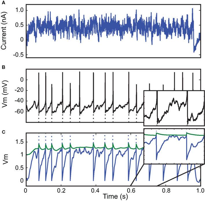
Figure 4. Fitting a leaky integrate-and-fire neuron with adaptive threshold to electrophysiological recordings. (A) A fluctuating in-vivo-like current was injected intracellularly in the soma of a L5 fast spiking cell. (B) The recorded spike train (black) is used to fit an adaptive threshold integrate-and-fire model. (C) Voltage trace (blue, no unit) and time-varying threshold (green) of optimized model. The gamma factor was 0.90 (precision δ = 2 ms).
Tables 1 and 2
report the results of fitting four different spiking models to the recordings in challenges A (regular spiking cell) and B (fast spiking cell). Each challenge includes the recordings of several identical trials (same input current; 13 trials in A and 9 trials in B), and we report the average and standard deviation for all quantities (gamma factor and parameter values). The recordings were divided into a training period (first 10 s), which was used to optimize the models, and a test period (last 10 s), which was used to calculate the gamma factors reported in the tables. We used the following values for the optimization algorithm: ω = 0.9, cl = 0.1, cg = 1.5. We used a local constant value much smaller than the global one so that the evolution of the algorithm is not dominated by the local term, which would make optimization slower.
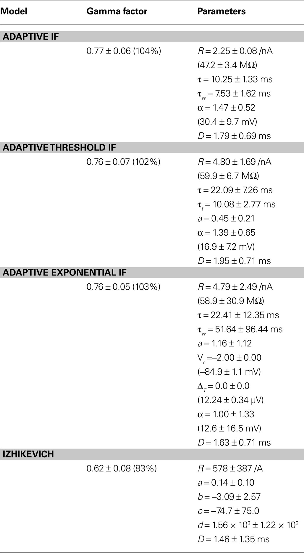
Table 2. Optimization results for Challenge B. Four neuron models were fitted to the electro-physiological recordings of an L5 fast spiking cell responding to in-vivo-like current injection. There were 9 trials with the same input.
Since only the spike trains were used for fitting, units were arbitrary (e.g. reset is 0 and threshold is 1 for the adaptive IF model). To interpret the parameter values, we also report scaled versions of the parameters obtained by changing the voltage units of the model in a such a way that the average and standard deviation of the model trace agree with those of the intracellular recording. The mean μd and the standard deviation σd of the experimental voltage trace were computed over the test period after the action potentials were cut. Then, the mean μm and the standard deviation σm of the voltage traces of the fitted model were also computed over the same test period. Finally, each parameter value X of the model was affine-transformed in either of the following two ways: Xtransformed = σd/σm ± (X − μm) + μd (for parameter Vr) or Xtransformed = σd/σm± X (for parameters α, ΔT, R).
Interestingly, for both challenges, best performance was achieved by a simple model, the integrate-and-fire model with adaptive threshold: Γ = 0.54 ± 0.05 for challenge A and Γ = 0.76 ± 0.07 for challenge B. The intrinsic reliability of the neurons can be defined as the average gamma factor between trials (Γin = 0.78 for challenge A and Γin = 0.74 for challenge B). Relative to the intrinsic reliability, the performance was 69% and 102% respectively. The fact that the performance on challenge B is greater than 100% probably reflects a drift in parameter values with successive trials, most likely because the cell was damaged. Indeed, the performance was tested on data that was not used for parameter fitting, so it could not reflect overfitting to noisy recordings but rather a systematic change in neuron properties. Consistently with this explanation, in both challenges the firing rate increased over successive trials (whereas the input was exactly identical). This change in neuronal properties was likely caused by dialysis of the cell by the patch electrode (the intracellular medium is slowly replaced by the electrode solution) or by cell damage.
A related model with an adaptive current instead of an adaptative threshold performed similarly. The performance of the adaptive exponential integrate-and-fire model (Brette and Gerstner, 2005
) (AdEx), which includes a more realistic spike initiation current (Fourcaud-Trocme et al., 2003
), was not better. This surprising result is explained by the fact that the optimized slope factor parameter (ΔT) was very small, in fact almost 0 mV, meaning that spike initiation was as sharp as in a standard integrate-and-fire model. The Izhikevich (2003)
model, a two-variable model with the same qualitative properties as the AdEx model, performed poorly in comparison.
Model Reduction
Our model fitting tools can also be used to reduce a complex conductance-based model to a simpler phenomenological one, by fitting the simple model to the spike train generated by the complex model in response to a fluctuating input. We show an example of this technique in Figure 5
where a complex conductance-based model described in benchmark 3 of Brette et al. (2007)
is reduced to an adaptive exponential integrate-and-fire model (Brette and Gerstner, 2005
). The complex model consists of a membrane equation and three Hodgkin-Huxley-type differential equations describing the dynamics of the spike generating sodium channel (m and h) and of the potassium rectifier channel (n). In this example, the gamma factor was 0.79 at precision 0.5 ms. This technique can in principle be applied to any pair of neuron models.
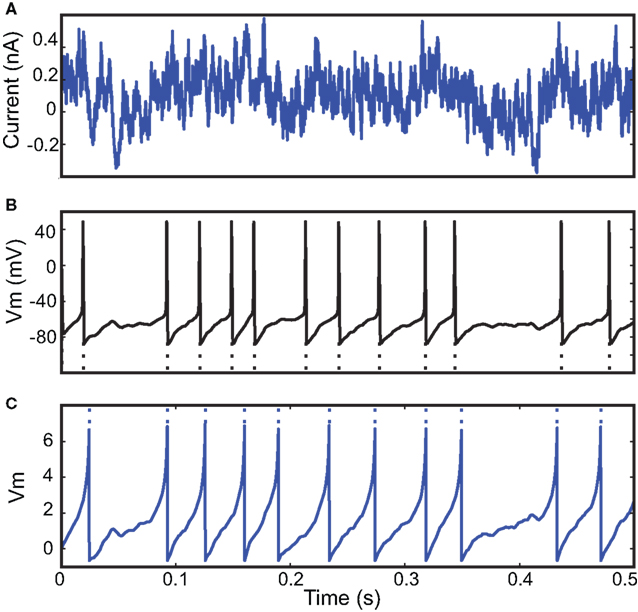
Figure 5. Model reduction from a Hodgkin−Huxley model to an adaptive exponential integrate-and-fire model (AdEx). (A) A 500-ms fluctuating current is injected into a conductance-based model. (B) The output spike train is used to fit an AdEx model. (C) Voltage trace of the optimized AdEx model. The gamma factor is 0.79 at precision 0.5 ms and the parameter values are τ = 12 ms, τw = 25 ms, R = 7.0 × 10⁹ A−1, VR = − 0.78, ΔT = 1.2, a = 0.079, α = 0 (normalized voltage units).
Benchmark
To test the scaling performance across multiple processors, we used a three machine cluster connected over a Windows network. Each computer consisted of a quad-core 64 bit Intel i7 920 processor at 2.6 GHz, 6 GB RAM, and an NVIDIA GeForce GTX 295 graphics card (which have two GPUs). The cluster as a whole then had 12 cores and 6 GPUs.
Performance scaled approximately linearly with the number of processors, either with CPUs (Figure 6
A) or GPUs (Figure 6
B). In the case of CPUs, performance was close to ideal (that is N processors performing N times faster than a single processor), and was slightly lower than ideal with GPUs. With our relatively inexpensive three machine cluster, we could achieve performance approximately 300 times faster than with a single CPU, allowing us to fit models in hours which would previously have taken weeks. A single GPU performed approximately 65× faster than a single CPU (or around 16× faster than the four cores available on a single machine in our cluster), and a dual-GPU GTX 295 card performed around 108× faster than a single CPU (or around 27× faster than the four CPUs alone).
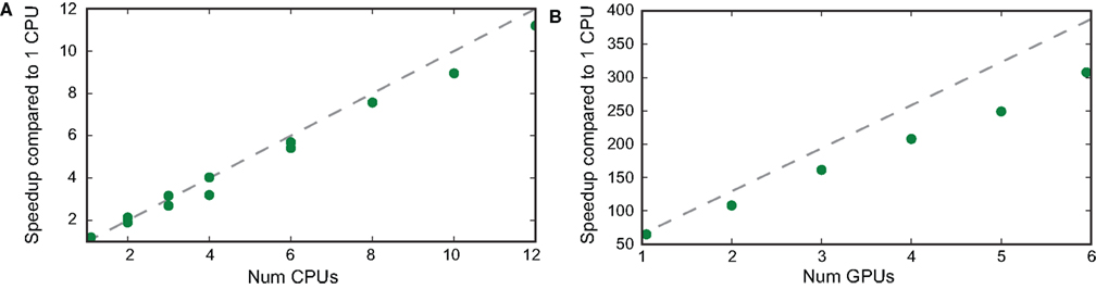
Figure 6. Speedup with multiple CPUs and GPUs. A fitting task was performed over 1-s-long electrophysiological data. (A) Speedup in the simulation of 10 iterations with 400,000 particles as a function of the number of cores, relative to the performance of a single CPU. We used different cluster configurations using 1−12 cores spread among one up to three different quad-core computers connected over a local Windows network. (B) Speedup in the simulation of 10 iterations with 2,000,000 particles as a function of the number of GPUs, relative to the performance of a single CPU (using the same number of particles). GPUs were spread on up to three PCs with dual-GPU cards (GTX 295).
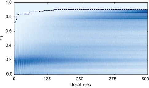
Figure 7. Evolution of the fitness values of particles during optimization. The color-coded background shows the distribution of the fitness values (Γ) of the 10,000 particles in each of the 500 iterations of the fitting procedure for trial 3 of challenge B (darker means higher density). The dotted line shows the gamma factor of the best particle. The neuron model was the adaptive threshold IF model. The best gamma factor reaches a plateau after 200 iterations but the other particles continue to evolve.
We presented vectorized algorithms for fitting arbitrary spiking neuron models to electrophysiological data. These algorithms can run in parallel on a graphics processing unit (GPU) or on multiple cores. It appeared that the speed improved by a factor of 50−80 times when the GPU was used for model simulations. With three dual-GPU cards, the performance was about 300 times faster than with one CPU, which makes it a cheap alternative to clusters of PCs. The algorithms are included as a model fitting library for the Brian simulator (Goodman and Brette, 2009
), which is distributed under a free open-source license
3
. This computational tool can be used by modellers in systems neuroscience, for example, to obtain empirically validated models for their studies.
We chose to use the particle swarm algorithm for optimization, but it can be easily replaced by any other global optimization algorithm that uses simultaneous evaluations of different parameter sets, such as genetic algorithms. Indeed, the optimization procedure is defined at script level (in Python) and runs on the main processor. The error criterion could also be modified, for example to include an error on the intracellular voltage trace, so that the model can predict both spike times and voltage.
Other model fitting techniques have been previously described by several authors, most of them based on maximum likelihood (Paninski et al., 2004
, 2007
). Our initial motivation for choosing a more direct approach based on general global optimization methods was that it applies to arbitrary models, including nonlinear ones, whereas maximum likelihood optimization is generally model-specific. Current maximum likelihood techniques apply essentially to linear threshold models, which constitute a large class of models but do not include, for example, the AdEx model and Izhikevich model, which we could evaluate with our algorithm. In Huys et al. (2006)
, a sophisticated maximum likelihood method is presented to estimate parameters of complex biophysical models, but many aspects of the model must be known in advance, such as time constants and channel properties (besides, the voltage trace is also used). Another important difference is in the application of these techniques. The motivation for maximum likelihood approaches is to determine parameter values when there is substantial variability in the neural response to repeated presentations of the same stimulus, so that model fitting can only be well defined in a probabilistic framework. Here, the goal was to determine precise spike times in response to injected currents in intracellular recordings, which are known to be close to deterministic (Mainen and Sejnowski, 1995
), so that probabilistic methods might not be very appropriate.
Our results on challenges A and B of the INCF Quantitative Modeling competition confirm that integrate-and-fire models with adaptation give good results in terms of prediction of cortical spike trains. Interestingly, the adaptive exponential integrate-and-fire model (Brette and Gerstner, 2005
) did not give better results although spike initiation is more realistic (Badel et al., 2008
). It appears that the fitting procedure yields a very small value for the slope factor parameter ΔT, consistent with the fact that spikes are sharp at the soma (Naundorf et al., 2006
; McCormick et al., 2007
). The Izhikevich model also did not appear to fit the data very well. This could be because spike initiation is not sharp enough in this model (Fourcaud-Trocme et al., 2003
) or because it is based on the quadratic model, which approximates the response of conductance-based models to constant currents near threshold, while the recorded neurons were driven by current fluctuations.
Our technique can also be used to obtain simplified phenomenological models from complex conductance-based ones. Although it primarily applies to neural responses to intracellular current injection, it could in principle be applied also to extracellularly recorded responses to time-varying stimuli (e.g. auditory stimuli), if spike timing is reproducible enough. An interesting extension, which could apply to the study of phase locking properties of auditory neurons, would be to predict the distribution of spike timing using stochastic spiking models.
The authors declare that the research was conducted in the absence of any commercial or financial relationships that could be construed as a potential conflict of interest.
This work was partially supported by the European Research Council (ERC StG 240132).