Neural circuit dynamics underlying accumulation of time-varying evidence during perceptual decision making
- 1 Program in Applied and Computational Mathematics, Center for the Study of Brain, Mind and Behavior, Princeton University, USA
- 2 Section of Neurobiology, Center for Perceptual Systems, Institute for Neuroscience, The University of Texas at Austin, USA
- 3 Howard Hughes Medical Institute, Department of Physiology and Biophysics, University of Washington, USA
- 4 Department of Neurobiology, Kavli Institute for Neuroscience, Yale University School of Medicine, USA
How do neurons in a decision circuit integrate time-varying signals, in favor of or against alternative choice options? To address this question, we used a recurrent neural circuit model to simulate an experiment in which monkeys performed a direction-discrimination task on a visual motion stimulus. In a recent study, it was found that brief pulses of motion perturbed neural activity in the lateral intraparietal area (LIP), and exerted corresponding effects on the monkeyquotidns choices and response times. Our model reproduces the behavioral observations and replicates LIP activity which, depending on whether the direction of the pulse is the same or opposite to that of a preferred motion stimulus, increases or decreases persistently over a few hundred milliseconds. Furthermore, our model accounts for the observation that the pulse exerts a weaker influence on LIP neuronal responses when the pulse is late relative to motion stimulus onset. We show that this violation of time-shift invariance (TSI) is consistent with a recurrent circuit mechanism of time integration. We further examine time integration using two consecutive pulses of the same or opposite motion directions. The induced changes in the performance are not additive, and the second of the paired pulses is less effective than its standalone impact, a prediction that is experimentally testable. Taken together, these findings lend further support for an attractor network model of time integration in perceptual decision making.
Introduction
Decision making involves accumulation of evidence about choice alternatives. This process often takes time when the quality of information is poor or there are numerous choice options to consider (Luce, 1986 ). In the past few years, experiments have revealed that such time integration is observable in single cortical neurons (Gold and Shadlen, 2007 ; Schall, 2001 ; Schall, 2003 ; Shadlen and Gold, 2004 ; Smith and Ratcliff, 2004 ). For instance, in a visual motion direction discrimination task, neurons in the lateral intraparietal (LIP) cortex of macaque monkeys exhibit slow ramping activity that is correlated with the formation of perceptual decisions about the direction (Roitman and Shadlen, 2002 ; Shadlen and Newsome, 2001 ). The difficulty of these decisions was varied from trial to trial by changing the percentage of dots moving coherently in one direction. Thus, at lower motion coherence, the subject's response time was longer, and the ramping of LIP neuronal firing rate was slower. Yet, for all levels of difficulty and for all reaction times, the firing rates reached the same level at the time the behavioral response was produced (Roitman and Shadlen, 2002 ).
We have previously investigated a biophysically realistic cortical network model of LIP responses in the random-dot motion direction discrimination experiment, and showed that this model could account for salient characteristics of the observed decision-correlated neural activity as well as the animal's accuracy and reaction times (Wang, 2002 ; Wong and Wang, 2006 ). In the model, slow recurrent excitation mediated by the N-methyl-D-aspartate (NMDA) receptors and feedback inhibition produce attractor dynamics which amplify the difference between conflicting inputs and generates a binary choice. One of the questions addressed in Wang (2002) was whether the model network can subtract negative signals as well as accumulate positive signals. Such a capability would be expected of an accurate neural integrator. It was shown that the attractor network model could indeed add and subtract inputs, but the influence of these inputs diminishes as a function of time, as the network converges toward one of the attractor states representing the alternative choices.
Recently, Huk and Shadlen (2005) investigated integration of time-varying evidence of opposite signs in the random-dot motion direction discrimination task. In addition to the moving random-dot pattern, a brief motion pulse in the background was introduced with a variable delay after the onset of the random dots. The direction of the motion pulse could be the same or opposite to the coherent motion of the random dots. On average, a motion pulse in the same (opposite) direction as the main motion stimulus resulted in more (less) choices in the direction of the coherent motion and faster (slower) decisions. Even though the perturbation from the motion pulse was brief, the ensuing changes in the firing rate of LIP neurons were sustained for several hundreds of milliseconds. Moreover, although the monkeys were trained to judge the direction of the random dots and to ignore the background pulse, the brief motion pulse had a long-lasting effect on the behavioral choices. Thus, this experiment lends support to the hypothesis that LIP neural activity is directly linked to time integration of evidence and perceptual decision in this task.
In the present paper, we examine whether the attractor network model is capable of reproducing the main observations of the motion pulse experiment of Huk and Shadlen (2005) . We report three main findings. First, we describe the decision dynamics of our recurrent cortical network model (Wong and Wang, 2006 ), when the input includes both a random-dot motion stimulus and targets which signal possible choices. Second, we show how the model accounts for the results in Huk and Shadlen (2005) . In particular, our model exhibits a violation of time-shift invariance (TSI), such that later pulses have weaker effects. Third, we introduce a novel protocol for testing time integration, using two motion pulses that are presented back to back within a trial. Our model makes testable predictions about the combined impacts of the double pulse on the temporal integration process. Part of this work has been presented in preliminary reports (Wong et al., 2005 , 2006 ).
Materials and Methods
The two-variable network model
In a previous paper (Wong and Wang, 2006 ), we reduced a spiking neuronal network model (Wang, 2002 ) to a two-variable model (see Figure 1 ) that could account for the experimental results of Shadlen and Newsome (2001) and Roitman and Shadlen (2002) . In the present work, we used this reduced model to further study motion integration in LIP neurons, with a focus on the experiment of Huk and Shadlen (2005) .
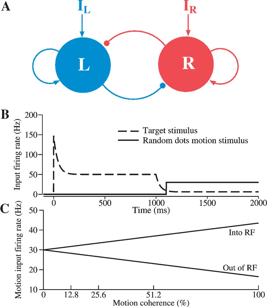
Figure 1. Schematic diagram of a reduced decision making network model. (A) The network consists of two units, representing two competing neural pools selective for leftward and rightward motion direction, respectively. Each is endowed with strong self-excitatory recurrent coupling (sharp arrowheads). Cross-coupling between the two units is effectively inhibitory (circular arrowheads) (through a shared inhibitory neural pool which is not explicitly represented in this reduced model). IL (IR) encompasses the external inputs from motion-selective (MT) neurons, target-sensitive neurons, and background neurons. (B) Inputs to the decision units within a trial consist of both target stimulus inputs (dashed line) and motion stimulus from the random-dots (bold line; shown here with zero motion coherence). According to the model, the target inputs are reduced when the random-dot motion appears because attention is directed to the motion. (C) The directional input comes from MT cells, whose firing rates depend linearly on motion coherence. Coherent motion toward (opposite) the response field, RF, increases (decreases) the cellquotidns output firing rate.
In the reduced network model, two competing neuronal pools (i = L, R) are selective for leftward (L) or rightward (R) direction of motion, respectively. The total synaptic input current Ii and the resulting firing rate ri of the neural population i obey the following input–output relationship

which captures the current–frequency function of a leaky integrate-and-fire neuron (Abbott and Chance, 2005 ). The parameter values are a = 270 Hz∕nA, b = 108 Hz, d = 0.154 second.
As schematically shown in Figure 1 , the neural circuit model is endowed with strong recurrent excitation, dominated by NMDA-mediated receptors within each pool of neurons. For simplicity here, we have neglected contributions by the AMPA receptors to local recurrent excitation. Hence the synaptic drive originating from the neural pool i is given by Si, which represents the fraction of the activated NMDA conductance. The two neural pools effectively inhibit each other through a third, common inhibitory neural population which is not explicitly described in the reduced model. Therefore, the total synaptic currents are
where the synaptic couplings are JLL = JRR = 0.3725 nA, JLR = JRL = 0.1137 nA. Imotion,i represents the random-dot stimulus. The dots provide evidence in favor of a saccade to one of the two choice targets. Itarget represents inputs due to choice targets. The choice targets are spots of light placed inside or outside the response field of the LIP neurons under study. Neurons also receive background synaptic inputs, with a mean of I0 = 0.3297 nA, and a fluctuating component given by a white-noise ηi(t) filtered by a synaptic time constant τnoise
with noise amplitude σnoise = 0.009 nA and filter time constant τnoise = 2 ms.
The network dynamics is dominated by Si, which has a slower time constant than the firing rate ri. The model is described by the following dynamical equations (cf. Appendix of Wong and Wang, 2006 ):

with γ = 0.641 and τS = 60 ms (Hestrin et al., 1990
). In this paper, we show network simulation results in terms of firing rates, which can be computed from the input–output relationship  .
.
Input implementation for targets and motion stimulus
The random-dot motion stimulus is represented by the output of neurons in the middle temporal (MT or V5) cortex which project to our LIP network model. Neurons in area MT are tuned to a particular direction of visual motion, and their firing rate are roughly a linearly increasing (decreasing) function of the motion coherence if the motion is in the preferred (null) direction of the cell (Britten et al., 1993 ). Specifically, we assume that the input current due to the random dots stimulus is
where c′ is the motion coherence,  , and the or − sign refers to the neural population for which the motion stimulus is the preferred or null direction, respectively. The pooled MT neuronal response to zero motion coherence is μ0 = 30 Hz (Britten et al., 1993
). The gain of MT firing rates on either preferred (null) direction f is chosen to be 0.45. We did not include a transient decay of the firing rates of MT cells during motion stimulus presentation (Priebe et al., 2002
).
, and the or − sign refers to the neural population for which the motion stimulus is the preferred or null direction, respectively. The pooled MT neuronal response to zero motion coherence is μ0 = 30 Hz (Britten et al., 1993
). The gain of MT firing rates on either preferred (null) direction f is chosen to be 0.45. We did not include a transient decay of the firing rates of MT cells during motion stimulus presentation (Priebe et al., 2002
).
The brief motion pulse, whenever presented, has a duration of 100 ms as in Huk and Shadlen (2005) , and an effective strength of p. We assumed p to be 11% coherence (cf. 10% in the modeling work in Huk and Shadlen, 2005 ). That is, p is 11% (−11%) if the motion pulse is in the preferred (null) direction of the cell.
Unlike the previous model simulations (Wang, 2002 ; Wong and Wang, 2006 ), in this work we explicitly include inputs for the targets which were used in the monkey experiment to indicate alternative saccadic responses. Specifically, during target presentation, large excitatory currents of the same amplitude were sent to both the leftward and rightward MT pools of neurons. This mimicks the experimental protocol of simultaneously presenting two targets in the response fields of the LIP neurons selective for the choice alternatives, before the motion stimulus is presented. LIP neurons exhibit strong responses to targets. Moreover, interestingly, LIP activity shows a brief decrease (a “dip”) immediately after the onset of the random dots stimulus, before the ramping of activity (Huk and Shadlen, 2005 ; Roitman and Shadlen, 2002 ). Such a dip has also been observed in other brain areas in monkey experiments (Li et al., 2006 ; Sato and Schall, 2001 ). To reproduce the dip phenomenon, we assume that upon the motion stimulus onset, there is a shift of attention from targets to the motion stimulus, leading to a general and equal reduction in the inputs to LIP from the upstream target coding neurons. Since visual information about the onset of random-dot motion affects LIP with latencies that are more than 100 ms, the target inputs fades before the motion input arrives (Huk and Shadlen, 2005 ; Kiani et al., 2006 ), as shown in Figure 2 A.
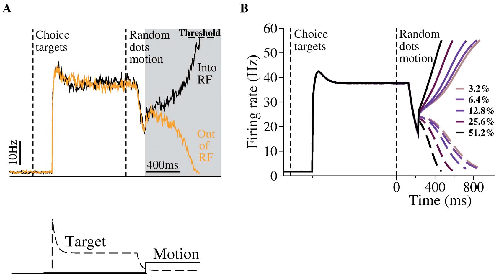
Figure 2. Neural dynamics of the decision network model. (A) Top: A sample trial with zero motion coherence. During target presentation, both neural pools (black and orange lines) achieve a relatively high steady state firing rate, similar to the observation of LIP neurons. During motion stimulus presentation (gray box), the firing rates of the two neural pools first increase together, then diverge over time, one ramping up whereas the other ramping down, resulting in a categorical choice (the decision bound is fixed at 55 Hz). Bottom: inputs. The target input represents static visual stimulus inputs with adaptation, as observed in experiments. The motion stimulus resembles the output firing rates of MT neurons. Note that in order to reproduce the ``dipquotidnquotidn immediately in neural activity immediately after motion stimulus onset, the target input is assumed to decrease (due to divided attention) after the motion stimulus onset but before the motion signals reach the LIP neurons. (B) Trial-averaged neural activities of the two neural pools with five motion coherence levels. Solid curves: winning population; dashed curves: losing population. Time courses of neural activity are aligned at the time of motion onset. Note slower ramping activity at a lower motion coherence. Only correct trials are shown.
The input current Itarget for target is implemented as
where ttarget and tmotion are the onset times for the targets and motion stimulus, respectively. This input current contains short-term adaptation with an exponential decay. The adaptation time constant of the neurons, τad, is chosen to be 40 ms. The transient attentional shift during motion stimulus presentation is indicated by a reduction in Itarget. The specific target input firing rates level are not important, as long as they are sufficiently large to allow the network to successfully transit from its low stable steady-state to its high symmetrical stable states. When the motion stimulus is presented, it is essential to reduce Itarget such that the overall input to the network is reduced, allowing competition between the two choice attractors (see section Results).
Data analysis
A decision is made whenever one of the two population firing rates reaches a prescribed threshold (or “decision bound”). It is set to be 55 Hz to fit the behavioral data of the no-pulse experimental data. To compute the reaction time, we have taken into account nondecision times (sensory input latency and motor response time). The overall nondecision latencies include latencies due to signal transduction from sensory cells to MT neurons (∼100 ms) (Britten et al., 1993 ); from MT neurons to LIP neurons (∼125 ms) (Huk and Shadlen, 2005 ); and finally from LIP neurons to the motor processing neurons for a saccadic movement (∼75 ms, compared with 100 ms in the modeling work of Huk and Shadlen, 2005 ). For simplicity, we assumed that the latencies are constant and independent of the decision. Thus, as in Huk and Shadlen (2005) , we have assumed that the latency from motion stimulus onset to LIP neurons is 225 ms. This means that, in simulations with brief pulse perturbations, our model LIP neurons are not affected by the motion pulse until 225 ms after the pulse onset.
Trial-averaged data were calculated with 1000 simulated trials. Trials were not taken into account if the decision threshold was crossed before motion pulse onset. Increasing the number of trials to 3000 did not substantially change the trial-averaged neural activities and the psychometric function. As in the experiment, all psychometric functions were fits of a logistic equation, P = 1∕( 1 exp [-(β0 β1c′)]), where P is the probability of making a preferred-target choice, and the β0 and β1 are fitted parameters. The amount of shift of the psychometric function was then computed from the difference in the β0 value.
Phase-plane analyses were done using XPPAUT (Ermentrout, 1990 ).
Results
Decision dynamics in the presence of targets
Figure 2 A shows the typical behavior of our network model. Upon presentation of the target input, both neural pools increase their activity and reach a relatively high steady-state firing rate. Such a high activity state corresponds to a symmetrical stable steady-state of our model (Wong and Wang, 2006 ). This high firing rate symmetric state is stable during target presentation, whereas a symmetric state at lower firing rate is unstable during motion stimulus presentation with zero coherence. This is because winner-take-all competition requires reverberatory excitation to amplify small fluctuations in the neural activities of the two decision pools. At high firing rates, the NMDAR-dependent synapses saturate (Wang, 1999 ), and cannot supply the necessary positive feedback to generate winner-take-all competition. This way, our model can account for both the stable symmetric state during target presentation and all-or-none decision making during stimulus presentation.
The targets create a large response in the network, and the model now captures the overall dynamics range of LIP firing rates more closely. In our previous work, we did not include the increase in LIP firing rates generated when the choice target is within the response field at the start of the trial. Here, we propose that this symmetric active state naturally represents the network state prior to the presentation of the moving dots. When the motion stimulus is presented, the decrease of the effective target input results in the loss of stability for this symmetric activity state. Driven by the motion stimulus, the two neural pools integrate the input signals and compete against each other. Eventually one of them climbs up while the other ramps down, leading to a categorical choice. Importantly, this is the case even with zero motion coherence (Figure 2 A) when the mean input is the same for the two neural pools. Noise inherent in the network determines the choice outcome in any given trial and the decision is at chance level across trials. Neural responses with nonzero motion coherence c′ are shown in Figure 2 B. It is clear that the ramping activity is faster at a higher c′.
Why is there winner-take-all competition during motion stimulus presentation but not when only the target input is present? The answer lies in the fact that the attractor landscape of the model network is reconfigured under different input conditions. One way to appreciate this is to study the phase-plane (Figure 3 ), in which the firing rates rR and rL are plotted against each other (Wong and Wang, 2006 ). At each of the epochs within a trial, when the input is fixed, the steady-states of the network can be obtained by setting the dynamical equations (Equation 2) of the network to be zero. For example, if we set dSL∕dt = 0, and solve for SL in −SL∕τ S (1 − SL) γ f[IL(SL, SR)] =0, we will obtain the so-called nullcline for SL (Strogatz, 2001 ). Similarly, we can also obtain the nullcline for SR. Converting Si back to ri, we can plot the nullclines in terms of the population firing rates in Figure 3 . The intersecting points of the two nullclines are the network's steady-states.
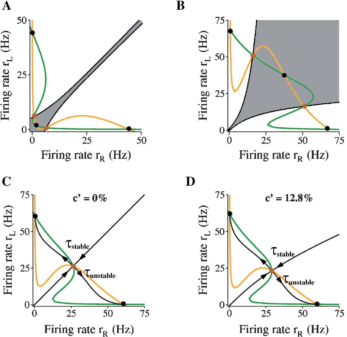
Figure 3. Decision attractor network is reconfigured during different epochs of a trial. In the phase-plane plot, orange and green lines are, respectively, nullclines of the population firing rates selective to leftward (rL) and rightward (rR) motion. Black (brown) filled circles are the stable (unstable) steady-states of the network. In (C) and (D), black lines with direction of arrows toward and away from the unstable steady-state (i.e., saddle point) are the stable and unstable manifolds of the saddle point. In the absence of noise, these manifolds determine the network dynamics. In (A) and (B), only the stable manifolds are plotted to show the multiple basins of attraction. Gray region is the basin of attraction of the spontaneous state in (A), or that of the symmetrical stable state in (B). (A) Without visual target nor motion stimulus input to decision network. (B) With target input only. Steady-states after adaptation. (C) With both (reduced) saccadic target input and motion stimulus of zero coherence. The stable time constant τstable (= 79 ms) toward the saddle unstable steady-state is about half that of the unstable time constant τunstable (= 175 ms). (D) With both (reduced) saccade target input and motion stimulus of 12.8% coherence. τstable = 77 ms and τunstable = 159 ms. See the text for more details.
As can be seen in Figure 3 A, in the absence of target or motion stimulus, there are three stable steady-states (black dots). One of them is the spontaneously active state (lower left corner, with a low rL = rR). The other two stable (off-diagonal) ones are persistently active states (rL is high and rR is low, or vice versa). The co-existence of these stable states endows the network with working memory capability: a transient stimulus can switch the network from the resting state to a persistent state which is self-sustained to hold information when the stimulus is withdrawn. Indeed, in prior studies (Roitman and Shadlen, 2002 ; Shadlen and Newsome, 2001 ), LIP neurons were selected on the criterion that they showed persistent activity during working memory. In the delayed response version of the motion direction discrimination task, a decision made during stimulus presentation can be stored in such a memory state and retrieved later to guide the behavioral response (Shadlen and Newsome, 2001 ; Wang, 2002 ; Wong and Wang, 2006 ). The regions of attraction of these stable states are bounded (in a noiseless system) by the black curves in Figure 3 A (see below for explanation).
When the two choice targets appear, both neural pools receive an identical strong input, and the configuration of the network changes. There is now a stable symmetrical steady-state at high firing rate (rL = rR ≃ 37.5 Hz) (Figure 3 B shows steady-state after adaptation). The equal excitation is strong enough to drive the state of the network from its initial low spontaneous state. This steady-state is presumed to be stable enough to prevent any decision making before the appearance of random-dots stimulus. Figure 3 B shows a large basin of attraction of this symmetrical state, confirming the stability of this state. In simulations, this state is always stable; the network never shifts to one of the choice attractors before onset of random-dot motion. Note that if the target inputs are sufficiently large, the two asymmetric states disappear, thus the only possible steady-state is the symmetric one and winner-take-all competition is no longer possible (Wong and Wang, 2006 ).
During motion stimulus presentation, the configuration of the network changes again such that now there exist only two stable and asymmetric steady-states. These are the decision or choice “attractors”. In Figure 3 C, the motion coherence is 0% and there is no net motion in either direction. Thus, because the overall inputs to both selective neural populations are equal, the phase-plane is symmetrical. When there is a bias in the net direction of the motion stimulus, the symmetry is broken, as illustrated in Figure 3 D with 12.8% of the random dots moving coherently to the left. In each case, the stable manifold of the saddle point (the “separatrix”) divides the phase-plane into two separate regions, the “basins of attraction” for the two decision attractors. In the absence of noise, if the network falls into one of the two basins, it will converge to the corresponding decision attractor. However, perceptual decisions are stochastic. The inclusion of noise in the model can break the symmetry even with zero motion coherence, so the network eventually converges to one of the two decision attractors in any given trial. However, the noise is not sufficiently large to push the system out of the stable state, before the motion stimulus is presented. With nonzero motion coherence, the basin of attraction is larger for the correct choice (with high rL in Figure 3 D) than for the erroneous choice (with high rR), therefore, the probability of correct responses becomes higher than the chance level.
Figures 4 A and 4 B show the time course of rL and rR at c′ = 0% and c′ = 12.8%. The corresponding phase planes are depicted in Figures 4 C and 4 D. During the motion stimulus, the network is forced to move toward one of the attractors such that the mean firing rates of the two competing neural pools eventually diverge over time. Whenever one of the firing rates (rL or rR) crosses a prescribed decision threshold (55 Hz in our case), a decision (L or R) is made and the corresponding response time is read out. The specific value of the threshold is chosen to fit the behavioral data of the experiment. In Figures 4 B and 4 D, the net direction of the motion stimulus was leftward. Therefore, the blue trajectory corresponds to the average correct choices while the red trajectory corresponds to incorrect choices.
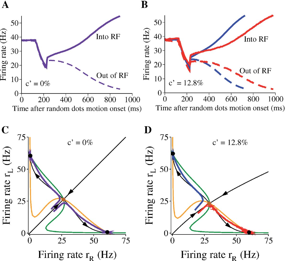
Figure 4. Network dynamics with two levels of motion coherence. Time course of neural responses and corresponding phase-plane plots during presentation of motion stimulus at c′ =0% (A,C) and c′ =12.8% (B,D). (A,C) Purple: trial-averaged neural activity after stimulus onset. Same for both selective pool of neurons, due to symmetry. (B,D) Blue: correct trials, red: error trials. In (C,D), black lines with arrows are the stable and unstable manifolds of the saddle point, respectively, and they control the flow of trajectories in the phase-plane in the absence of noise. Note that with a nonzero motion coherence, the temporal dynamics are slower on error trials (red) than on correct trials (blue) (B). In the phase-plane (D), the networkquotidns trajectory on error trials passes by the saddle point where the dynamics are slow. Each trajectory or time course is the average over 1000 trials.
Comparing Figures 4 A and 4 B, and also in Figure 2 , we can see that the ramping time course is generally faster at higher coherence. Moreover, given a fixed motion coherence (Figure 4 B), the neural dynamics are slower on error trials (red curves) than on correct trials (blue curves). This can be understood in the phase-plane plot (Figure 4 D). In error trials, the trajectory has to cross the separatrix of the saddle point so that it eventually converges to the “wrong attractor” (with a high rR in this example). This implies that the trajectory follows the stable manifold for a while, and then passes very near the saddle point, where the network dynamics are slower (see Wong and Wang, 2006 for explanation). The behavioral implication is that reaction times are slower on error trials than on correct trials, consistent with the observations in the monkey experiment (Roitman and Shadlen, 2002 ).
Temporal integration of a brief pulse of sensory evidence
After re-evaluating the dynamics of the attractor model with the addition of target input, we next study how the model can integrate an additional brief motion stimulus. We used the same task protocol as in Huk and Shadlen (2005) , in which a 100 ms motion pulse was applied after a time delay from motion stimulus onset (see Figure 5 ). The direction of the pulse could be the same as or opposite to that of the coherent motion of the random dots, which will be referred to as positive and negative, respectively. As in the experiment, we varied the onset times of the motion pulse to be 100, 150, 211, 287, and 392 ms after motion stimulus onset.
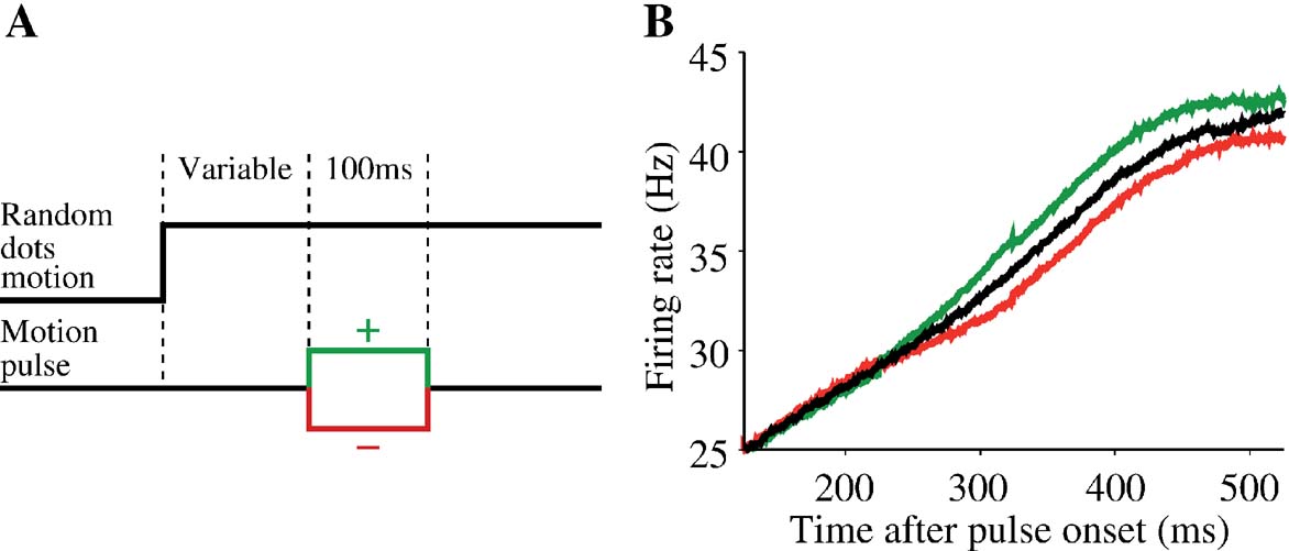
Figure 5. Single motion pulse results in persistent change of neural response in the model. (A) After motion stimulus onset, a 100 ms pulse is presented either in the same (green) or opposite (red) direction as the coherent random-dot motion. As in the experiment of Huk and Shadlen (2005), five different motion pulse onset times were used: 100 , 150, 211, 287, and 392 ms after motion stimulus onset. (B) Pulse onset is 100 ms after onset of a c′ =12.8% motion stimulus. The neural traces are trial-averaged firing rates in trials when the choice is the preferred direction of the cell. Only correct trials are shown here. Black: no motion pulse; green: positive pulse; red: negative pulse. All firing rate traces shown are truncated at the time the decision threshold is crossed, hence the apparent saturation of firing rates due to averaging effect near threshold. A pulse takes 225 ms to reach the decision neurons, and the induced change in the neural activity persists even after pulse is switched off.
In general, we expect a good integrator to be able to add or subtract additional sensory evidence, thereby enhancing or reducing the probability of a given decision outcome. A motion pulse in the direction of the coherent motion should result in more likely choices in that direction and faster decisions. Conversely, a motion pulse in the direction opposite the coherent motion should result in less accurate and slower decisions. As an example, Figure 5 B shows, for a fixed motion coherence and pulse onset time, the impact of a motion pulse on trial-averaged population firing rate when the choice is correct and in the response field. The pulse (100 ms after motion stimulus onset) is in the same (green) or different (red) direction as that of the coherent motion. We see from the figure that, on average, the motion pulse perturbs the ramping dynamics of the population firing rates. A positive pulse increases the time course of firing rates (green) compared with the time course without motion pulse (black). Conversely, a negative pulse decreases the firing rates (red). The change in the neural activity persists longer than the duration of the pulse itself, a hallmark of neural integration. Hence, the small amount of evidence is integrated and remembered to influence the perceptual choice that takes place later in time. This is also true for changes of neural activity averaged over a range of motion coherence levels (Figure 6 B), which reproduces the main physiological observation of Huk and Shadlen (2005) (reproduced in Figure 6 A). Note that these changes in neural activity converge over time, because the neural firing rates are truncated at the same decision threshold with or without a motion pulse.
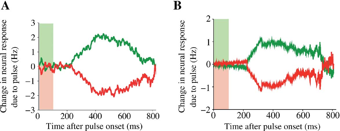
Figure 6. Mean persistent change of neural activity due to a brief motion pulse. Effects of a pulse perturbation, averaged over all trials, motion coherence levels and pulse onset times. A single pulse of 100 ms duration induces a long-lasting change in the trial-averaged neural activity in both the experiment (A) and in the model simulation (B). Green: positive pulse; red: negative pulse. Colored light green (red) bars denote the duration of the positive (negative) motion pulse (panel A is reproduced from Huk and Shadlen (2005) with permission.)
These persistent changes in neural activity induced by brief motion pulse also led to effects on behavior. For example, with a motion coherence of c′ = 12.8% (Figure 5 B), a positive pulse changes the accuracy and mean reaction time from 95.2% and 746 ms, respectively, to 97.1% and 714 ms. Conversely, a negative pulse decreases the accuracy to 88.7% and prolongs the mean reaction time to 783 ms.
Averaging over all five pulse onset times, the net effect of a motion pulse is a shift in both the psychometric function and the mean reaction times (Figure 7 ). The psychometric function is shifted by ∼ 1.6%, as in Huk and Shadlen (2005) . Note that these are the mean effects of five motion pulses at different time points. As we shall see below, the effect of pulse perturbation is larger with an earlier onset time. Thus, we have shown that the attractor model, like the diffusion model (Huk and Shadlen, 2005 ), is capable of reproducing these behavioral and neurophysiological data of Huk and Shadlen (2005) .
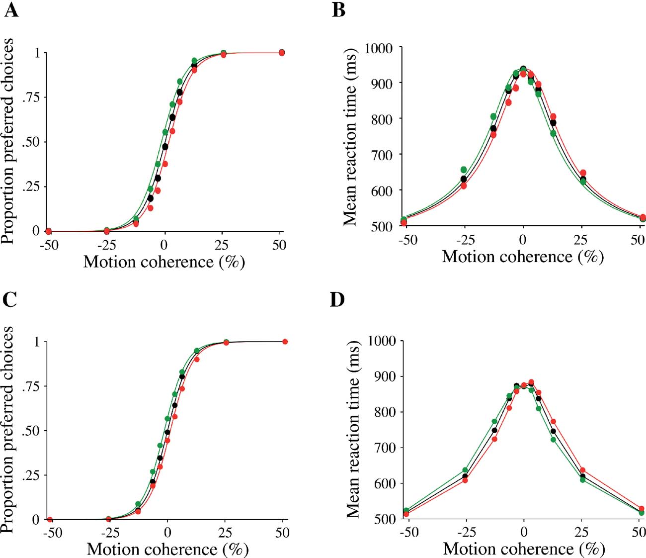
Figure 7. Effect of a motion pulse on decision accuracy and reaction time of the model. Choices (A,C) and mean reaction times (B,D) are shown as function of the motion coherence. Black: no motion pulse. Green (respectively red): a positive (respectively negative) pulse shift the psychometric and chronometric functions leftward (respectively rightward). (A,B) Data from experiments (reproduced from Huk and Shadlen (2005) with permission); (C,D) model simulations. Psychometric function is fitted by a logistic function (see section Materials and Methods). Curves were calculated by averaging over pulses of five different onset times.
Violation of TSI
When the data from our simulations are sorted according to the pulse onset times, it is apparent that the effect of the pulse is weaker when its onset time is later (Figure 8 ). This diminution in impact is apparent for both the neural responses (Figure 8 A) and choice behavior (Figure 8 B) produced by our model. This is clearly a violation of the invariance in time-translation termed TSI, similar to the violation observed in the Huk and Shadlen (2005) experiment.
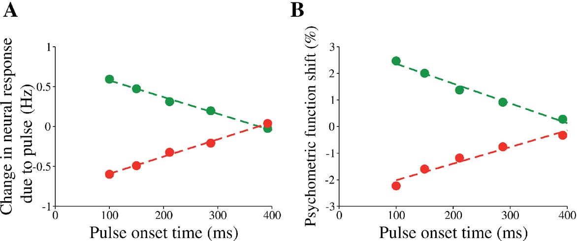
Figure 8. Violation of TSI: weaker influence of a later pulse on neural activity and choice accuracy in the model. (A) Average instantaneous change in neural firing rate as a function of the pulse onset time. The instantaneous change is calculated from 250 to 350 ms after pulse onset, as in the experiment. The green (red) trace denotes the change in firing rates due to positive (negative) pulse. Only data from trials with weak motion coherence of 0 and 3.2% were used. (B) Shift in psychometric function decreases with increased pulse onset time. Psychometric function shift is calculated from the shift of the fitted logistic functions (see section Materials and Methods). Standard errors are small, and hence omitted.
To provide an intuitive explanation of the TSI violation, consider a cartoon in which the decision making network is described by an energy function of neural firing rate, or a “potential well” (Figure 9 ). The minima of the well denote the stable steady-states (attractors), and the local maximum is the unstable steady-state that divides the basins of attraction. When the motion stimulus is presented, the network changes its configuration, and its dynamics is represented as a ball rolling toward one of the minima. The shallower the potential well (near the unstable steady-state), the slower the ramping activity. A positive (negative) motion pulse would give the network a brief kick, causing the integration to increase (decrease) its rate of ramping. With these nonlinear potential wells, one can easily see that the network states can differ, depending on the stage in a trial. If the pulse onset is not early enough, the network state has time to accelerate away from the unstable point and it becomes harder for the pulse to exert an effect on the network. This explains, qualitatively, the violation of TSI.
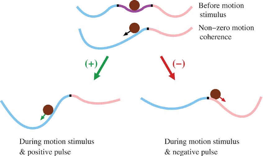
Figure 9. Effect of motion pulse on a nonlinear attractor network. Diagram depicts a network whose dynamics are described by an energy function (or potential well) of the neural firing rate. The speed of the temporal dynamics is proportional to the slope of the potential well, and the steady-states correspond to the minima and maxima (where the slope is zero). Magenta, blue and pink regions denote the basins of attractions. Each black mark denote the unstable steady-state that separates the two neighboring basins of attraction. The brown ball represents the instantaneous state of the network. Configurations of the network before motion stimulus presentation (top), and during motion viewing with a low motion coherence (middle) favoring the blue choice attractor. The black arrow indicates that the network is more inclined to move toward the blue attractor. When a positive motion pulse is added, the blue decision state has a deeper basin of attraction than before. Therefore, the network dynamics exhibit a faster ramping speed toward the blue state (bottom, left). When a negative motion pulse is presented instead, the blue decision state becomes less attractive while the pink decision state becomes more attractive (bottom, right). This results in a network state less inclined to move to the blue attractor. Green (red) arrow on the ball represents the average effect of a positive (negative) pulse on the network dynamics. With later motion pulse onset, the network becomes harder to influence since it is more likely to have commenced acceleration toward one of the choice attractors, thereby violating TSI. Not shown in the figure is that the ball is always under the continuous influence of noisy perturbations.
Reverberation, not leak, gives rise to the observed violation of TSI
To shed further insights into the violation of TSI, we contrast two possibilities: a leaky, stable accumulator of the variety incorporated in some diffusion models (Usher and McClelland, 2001 ) and an attractor dynamical model characterized by strong recurrent excitation. One might wonder whether the addition of a leak to a diffusion-like model, and thus a finite integration time, could contribute to the violation of TSI. In fact, intuitively one expects that a leak would lead to a violation of TSI in the opposite direction, namely the impact of a brief pulse should be larger with a later onset time, contrary to the experimental observation. This is because an earlier pulse is gradually “forgotten” due to the leak and does not affect significantly the decision that occurs much later (Kiani et al., 2006 ).
To check this intuition, we analyzed a simple linearized version of our model. For simplicity, let us assume that during an unbiased (c′ = 0%) motion stimulus presentation, the slow ramping dynamics are roughly along the unstable manifold of the saddle point. Therefore, the overall dynamics can be approximated by a single variable S = SL − SR (see Supplemental Data in Wong and Wang, 2006 ). We shall also neglect the effects of noise. Then we can approximate the network dynamics by
where Sss and τ are the effective steady-state and time constant of the network, respectively. p(t) is a step function of constant height p from t = T to t = T Tp, that denotes the perturbation due to a motion pulse. The pulse height p can be positive or negative, denoting whether the pulse is adding or subtracting evidence to the coherent motion.
This is a linear dynamical equation with a time-dependent input p(t), which can be readily solved analytically. The change ΔS in S due the pulse p(t) is
Because of the factor e−t∕τ , we expect that the sustained change due to a pulse to decay over time. On the other hand, for a fixed pulse duration Tp, the factor eT∕τ is a monotonically increasing function of the pulse onset time T, in support of the above intuitive reasoning. However, if the pulse is presented too late, the pulse effect should start to decrease, because now the ramping activity is truncated when the decision threshold is reached.
In the limit of largeτ, as in a perfect integrator (diffusion) model,
which is independent of the pulse onset time T, but dependent on the integral (total area) of the pulse pTp. This result is consistent with our initial hypothesis that the effect of a fleeting motion pulse on a perfect integrator (or a diffusion model) is time-shift invariant.
This analysis is valid for a stable leaky integrator processes. If the integrator is exponentially unstable, e.g., resulting from reverberating excitation in a recurrent network, then the system is described by
in which case the pulse effect becomes

Therefore, the change in the activity decreases with pulse onset time, consistent with our model simulations. Note that in our nonlinear network model the reverberating excitation is ultimately counterbalanced by negative feedback or saturation, which is not included in this simplified linear analysis. Nevertheless, the argument explains why our attractor circuit violates TSI as observed experimentally (Huk and Shadlen, 2005 ). This suggests that LIP embodies a recurrent circuit mechanism for time integration during perceptual decision making.
Model predictions with two motion pulses
We noted that pulses shown at different time during motion stimulus may induce nonlinear effects as a result of truncation of the firing rate at the decision bound. Thus, it would be desirable to use other protocols for testing nonlinearities of neural integration that avoid the decision threshold effect. To this end, we developed and analyzed a novel protocol that consists of two motion pulses (Figure 10 ). The first motion pulse is immediately followed by a second pulse which has the same magnitude and duration but could either be of the same or opposite motion direction as the first pulse. Hence, there are four possible combinations, depending on the signs of the two pulses. We have limited ourselves to early onset times for the double-pulse, before threshold crossing becomes more likely to occur.
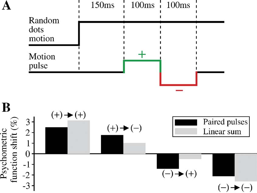
Figure 10. Nonlinearities in time integration using a double-pulse protocol. (A) A positive pulse is immediately followed by a negative pulse of the same magnitude but opposite direction. In principle, there are four possible combinations of the two pulses: positive → positive, positive → negative, negative → positive, negative → negative. (B) Two pulses, each of 100 ms duration, are presented at 150 and 250 ms after motion stimulus onset. Shift of the psychometric function for each of the four possible paired-pulse combinations (black bar) is compared to the linear sum of the shifts due to two individual pulses (gray bar). The second pulse in the paired-pulse protocol has a weaker effect than its standalone counterpart. In the (+)→(+) and (−) →(−) pairs, the double pulse is weaker than the sum of the effects produced by the two pulses on their own. In the (+)→(−) and (−) →(+) pairs, the first pulse controls the sign of the effect. The sum of single pulse effects would be cancelation were it not for the violation of TSI. There is less cancelation by the second pulse in the double-pulse protocol.
We examined in the model how a pair of pulses affects the psychometric function. The shift in psychometric function is then compared with the linear sum of the shifts caused by the two individual pulses that make up the paired pulses, presented alone. We chose the onset times of 150 and 250 ms for the pair of pulses, which allowed us to distinguish most clearly between the effect of the paired pulses and that of the sum of two single pulse perturbations. The results are shown in Figure 10 . For each of the four possible combinations of paired pulses, the effect of the double pulse is shown by the resulting shift of the psychometric function relative to one obtained without any motion pulses (Figure 10 B, black bar). The effect has units of equivalent motion strength. We also derived the shift of the psychometric function for each of the individual pulses, presented on their own. We added these individual shifts for pairs corresponding to same 2-pulse configurations (Figure 10 B, gray bar). It is clear that the effect of the double pulse is not the same as the sum of the individual pulses. Consider the pulse combinations with opposite sign. Were it not for the violation of TSI, we would expect the sum of individual pulse effects to cancel exactly. However, because the process is not TSI, the effect of the later pulse is not large enough to cancel the first. In the double-pulse protocol, however, this effect is magnified: the effect is dominated by the first pulse. For pulses of the same sign, the same logic applies. In the double-pulse protocol, the effect of second pulse is attenuated. Therefore, we see a smaller effect here than the sum of the individual pulse effects.
Figure 11 shows changes in the neural activity induced by two pulses of opposite signs, compared to those by a single pulse. In this example, the second pulse does not completely cancel out the effect of the first pulse, and the net persistent change (before the decision threshold effect becomes important) caused by the paired pulses is not zero. Therefore, the paired-pulse protocol provides another demonstration that the network dynamics is not time-shift invariant, even when the effect of decision threshold crossing is negligible.
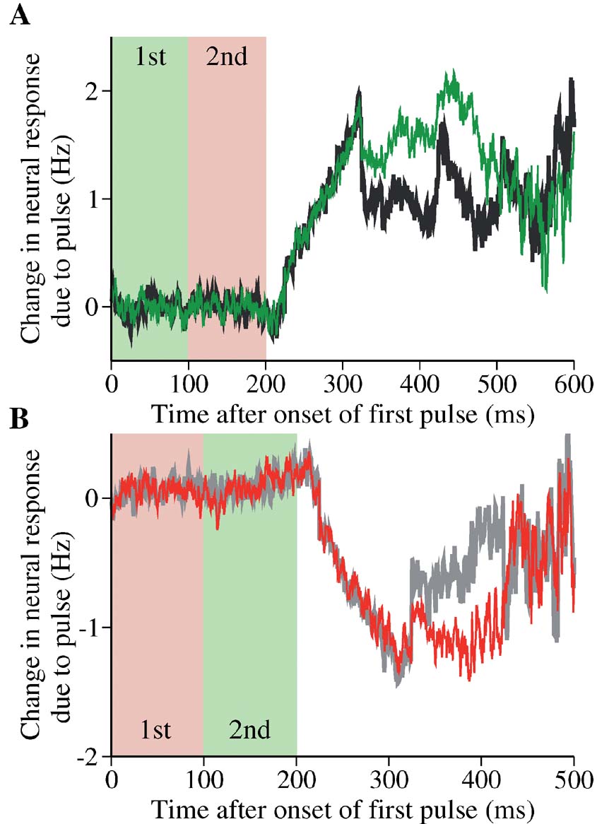
Figure 11. Changes in the neural response by paired pulses in the model. (A) Black: a positive pulse is followed by a negative pulse. The time course of neural activity is compared with that produced by a single positive pulse (green). Light green and pink regions represent the duration of the first and second pulse, respectively. Effectively, the second pulse in the double pulses is unable to completely suppress the change caused by the first pulse. Because of the input latency of 225 ms, the neural response to the first pulse occurs in the time window from 225 to 325 ms, and to the second pulse from 325 to 425 ms. Motion coherence is 12.8% in the neuronquotidns preferred direction. (B) Gray: a negative pulse is followed by a positive pulse. The time course of neural activity is compared with that produced by a single negative pulse (red). Same label convention as in (A). The second positive pulse does not suppress the change due to the first negative pulse. Motion coherence is 25.6%. The neural responses were obtained in correct trials when the choice is the preferred direction. In both panels, the difference in the neural response is measured with respect to the average of trials without pulses that lead to the same correct choice.
Discussion
In this paper, we further tested a recurrent neural circuit model of perceptual decision making, investigating how brief pulses of motion are temporally integrated. We found that the model was able to replicate both the psychophysical and neural data of the motion pulse experiments in Huk and Shadlen (2005) .
Unlike our previous modeling work (Wang, 2002 ; Wong and Wang, 2006 ), here we explicitly represented the presence of the choice targets as inputs. This facilitated a comparison of the time course of neural activity between the model and the experiment. Interestingly, the inclusion of target inputs renders the model behavior closer to a one-dimensional model of the decision process. Indeed, in the analysis of Wong and Wang (2006) , we found that the network dynamics in response to the motion stimulus displays two phases over time, which are roughly associated with the trajectory along the stable and unstable manifolds of a saddle point. In a linear description that assumes that the networkquotidns decision process takes place close to the saddle point, the ramping neural activity is dictated by two time constants (τstable and τunstable) associated with the stable and unstable manifolds of the saddle point. The time constant τstable was a few hundreds of milliseconds, and hence not negligible, implying that the network must be described by two dynamical variables. In the present work, when the target inputs are included, the neural firing rates are high at the onset time of the motion stimulus, and the network's phase-plane configuration is different. In this case, the recurrent excitation resulting from increasing neural firing significantly shortened τstable, which is now less than 100 ms and about half of τunstable (see Figure 3 ). Therefore, with the help of the target inputs, it is more plausible to approximate the network behavior by a one-dimensional dynamical system, roughly along the unstable manifold of the saddle point (Bogacz, 2007 ; Bogacz et al., 2006 ; Brown and Holmes, 2001 ). We emphasize, however, that this reduced system is still a nonlinear attractor model in which strongly recurrent neural dynamics play a key role in decision computations, in contrast to the linear diffusion model (Ratcliff and Smith, 2004 ; Smith and Ratcliff, 2004 ; Mazurek et al., 2003 ).
We designed our model to replicate a dip of neural firing at the onset of the motion stimulus, as observed in LIP neurons (Huk and Shadlen, 2005 ; Roitman and Shadlen, 2002 ). Such a pause in neural activity has been observed in the frontal eye fields (Sato and Schall, 2001 ) and superior colliculus (Li et al., 2006 ). We hypothesize that this dip results from “divided attention”, i.e., the subject's covert attention is shifted to the motion stimulus, and therefore the effective signal representing the targets is reduced. Alternatively, the dip could represent some sort of “reset” of neural integrators before the integration process, and is independent of the duration of the motion viewing time (Kiani et al., 2006 ).
The attractor circuit model replicated the experimentally observed violation of TSI. It explains the diminishing effect of a pulse as time elapses during the decision process. In our model simulations, the change in neural activity due to a pulse (Figure 6 B) is slightly smaller than the LIP data (Figure 6 A, reproduced from Huk and Shadlen, 2005 ). The small discrepancy is not surprising, because we did not attempt to fully optimize the model parameters to fit the experimental data quantitatively. Nonetheless, our model appears to provide a good explanation for the degree to which later pulses exert diminishing effects on the decision. This trend is not readily reproducible with the diffusion model, even taking into account the nonlinearity due to crossing of a decision threshold (Huk and Shadlen, 2005 ). Furthermore, we demonstrated that this trend is not explained by a leaky integration process. A more detailed theoretical study of this issue will be reported elsewhere. Therefore, our result lends further support to the reverberating circuit model.
Alternative explanations are conceivable. For instance, it is possible that the decision threshold is not fixed but decreases in time, presumably as a result of an urgency signal in the brain that becomes stronger later in a trial (Churchland et al., 2007 ; Ditterich, 2006 ; Hanks et al., 2007 ; Reddi and Carpenter, 2000 ). Qualitatively this would be equivalent to acceleration of the ramping activity (while the decision threshold is fixed), which naturally results from recurrent excitatory dynamics as in our attractor model.
To differentiate a linear diffusion-like model with a fixed decision bound and a nonlinear recurrent circuit model, the single-pulse protocol is not ideal because the truncation of firing rate by a decision threshold inevitably introduces nonlinear effects. We proposed a double-pulse protocol, in which two brief pulses are presented consecutively in time, relatively early in a trial to avoid the thresholding effect. This protocol reveals nonlinear dynamics in the process of time integration subserved by recurrent neural circuit dynamics. We think it might help to differentiate the model proposed here from alternative models such as the diffusion model with a collapsing bound or urgency.
In a broader context, this modeling work represents an attempt to link the principles derived from experimental studies to more realistic neural networks. The body of experimental work on the neurobiology of decision making tends to rely on abstract formalisms to relate neural activity with decisions. In recent years, biophysically based neural circuit models have been developed and shown to yield similar results as, but also some differences from, the drift-diffusion models. Furthermore, tools such as signal detection theory, wave difference theory and diffusion models (Gold and Shadlen, 2007 ; Link, 1992 ; Ratcliff and Rouder, 1998 ; Ratcliff and Smith, 2004 ; Smith and Ratcliff, 2004 ) do not address the neural circuitry that underlies the process. The level of modeling represented in this study translates the principle of bounded integration into a mechanism that is more easily reconciled with real cortical circuits (Lo and Wang, 2006 ; Machens et al., 2005 ; Miller and Wang, 2006 ; Wang, 2002 ; Wong and Wang, 2006 ). We expect these insights to lead to more refined experimental tests.
Conflict of Interest Statement
The authors declare that the research was conducted in the absence of any commercial or financial relationships that could be construed as a potential conflict of interest.
Acknowledgements
Part of this work was done when both K.-F. W. and X.-J. W. were both at Brandeis University and were supported by NIH grants MH062349 and DA016455, and by the Swartz Foundation. A. C. H. is supported by The University of Texas at Austin SRA. M. N. S. is supported by HHMI, EY011378, and RR0016639. We would like to thank Philip Eckhoff, Phil Holmes, and Christian Luhmann for careful reading of the manuscript.
References
Abbott, L. F., and Chance, F. S. (2005). Drivers and modulators from push-pull and balanced synaptic input. Prog. Brain Res. 149, 147–155.
Bogacz, R. (2007). Optimal decision-making theories: linking neurobiology with behaviour. Trends Cogn. Sci. 11, 118–125.
Bogacz, R., Brown, E., Moehlis, J., Holmes, P., and Cohen, J. D. (2006). The physics of optimal decision making: a formal analysis of models of performance in two-alternative forced choice tasks. Psychol. Rev. 113, 700–765.
Britten, K. H., Shadlen, M. N., Newsome, W. T., and Movshon, J. A. (1993). Response of neurons in macaque MT to stochastic motion signals. Vis. Neurosci. 10, 1157–1169.
Brown, E., and Holmes, P. (2001). Modeling a simple choice task: stochastic dynamics of mutually inhibitory neural groups. Stoch. Dyn. 1, 159–191.
Churchland, A. K., Kiani, R., and Shadlen, M. N. (2007). LIP neurons combine accumulated evidence with a representation of elapsed time -urgency- to mediate a perceptual decision. Soc. Neurosci. Abstract no. 507.3 .
Gold, J. I., and Shadlen, M. N. (2007). The neural basis of decision making. Annu. Rev. Neurosci. 30, 535–574.
Hanks, T. D., Kiani, R., Kira, S., and Shadlen, M. N. (2007). Evidence for the incorporation of psychophysical urgency in decision making. Soc. Neurosci. Abstract no. 507.4 .
Hestrin, S., Sah, P., and Nicoll, R. A. (1990). Mechanisms generating the time course of dual component excitatory synaptic currents recorded in hippocampal slices. Neuron 5, 247–253.
Huk, A. C., and Shadlen, M. N. (2005). Neural activity in macaque parietal cortex reflects temporal integration of visual motion signals during perceptual decision making. J. Neurosci. 25, 10420–10436.
Kiani, R., Hanks, T. D., and Shadlen, M. N. (2006). Improvement in sensitivity with viewing time is limited by an integration-to-bound mechanism in area LIP. Soc. Neurosci. Abstract no. 605.7.
Li, X., Kim, B., and Basso, M. A. (2006). Transient pauses in delay-period activity of superior colliculus neurons. J. Neurophysiol. 95, 2252–2264.
Lo, C.-C., and Wang, X. J. (2006). Cortico-basal ganglia circuit mechanism for a decision threshold in reaction time tasks. Nat. Neurosci. 9, 956–963.
Luce, R. D. (1986). Response times: their role in inferring elementary mental organization (Oxford Psychology Series, 8) (New York, Oxford University Press).
Machens, C. K., Romo, R., and Brody, C. D. (2005). Flexible control of mutual inhibition: a neural model of two-interval discrimination. Science 18, 1121–1124.
Mazurek, M. E., Roitman, J. D., Ditterich, J., and Shadlen, M. N. (2003). A role for neural integrators in perceptual decision making. Cereb. Cortex. 13, 1257–1269.
Miller, P., and Wang, X. J. (2006). Inhibitory control by an integral feedback signal in prefrontal cortex: a model of discrimination between sequential stimuli. Proc. Natl. Acad. Sci. USA 103, 201–206.
Priebe, N. J., Churchland, M. M., and Lisberger, S. G. (2002). Constraints on the source of short-term motion adaptation in macaque area MT. i. the role of input and intrinsic mechanisms. J. Neurophysiol. 88, 354–369.
Ratcliff, R., and Rouder, J. N. (1998). Modeling response times for two-choice decisions. Psychol. Sci. 9, 347–356.
Ratcliff, R., and Smith, P. L. (2004). A comparison of sequential sampling models for two-choice reaction time. Psychol. Rev. 111, 333–367.
Reddi, B. A., and Carpenter, R. H. S. (2000). The influence of urgency on decision time. Nat. Neurosci. 3, 827–830.
Roitman, J. D., and Shadlen, M. N. (2002). Response of neurons in the lateral intraparietal area during a combined visual discrimination reaction time task. J. Neurosci. 22, 9475–9489.
Sato, T., and Schall, J. D. (2001). Pre-excitatory pause in frontal eye field responses. Exp. Brain Res. 139, 53–58.
Schall, J. D. (2003). Neural correlates of decision processes: neural and mental chronometry. Curr. Opin. Neurobiol. 13, 182–186.
Shadlen, M. N., and Gold, J. I. (2004). The neurophysiology of decision-making as a window on cognition. In The Cognitive Neurosciences, 3rd edn, M. S. Gazzaniga, ed. (Cambridge, MA, MIT).
Shadlen, M. N., and Newsome, W. T. (2001). Neural basis of a perceptual decision in the parietal cortex (area LIP) of the rhesus monkey. J. Neurophysiol. 86, 1916–1936.
Smith, P. L., and Ratcliff, R. (2004). Psychology and neurobiology of simple decisions. Trend Neurosci. 27, 161–168.
Strogatz, S. H. (2001) Nonlinear dynamics and chaos: with applications to physics, biology, chemistry and engineering (Cambridge, MA, Perseus Books Group) .
Usher, M., and McClelland, J. L. (2001). On the time course of perceptual choice: The leaky competing accumulator model. Psychol Rev. 108, 550–592.
Wang, X.-J. (1999). Synaptic basis of cortical persistent activity: the importance of NMDA receptors to working memory. J. Neurosci. 19, 9587–9603.
Wang, X.-J. (2002). Probabilitic decision making by slow reverberation in cortical circuits. Neuron 36, 955–968.
Wong, K.-F., Huk, A. C., Shadlen, M. N., Wang, X.-J. (2005). Time integration in a perceptual decision task: adding and subtracting brief pulses of evidence in a recurrent cortical network model. Soc. Neurosci. Abstract no. 621.5.
Wong, K.-F., Huk, A. C., Shadlen, M. N., Wang, X.-J. (2006). Time integration in a perceptual decision task: adding and subtracting brief pulses of evidence in a recurrent cortical network model. Cogn. Syst. Neurosci. Abstract no. 177.
Keywords: intraparietal cortex, reaction time, computational modeling, attractor network, visual motion discrimination
Citation: Kong-Fatt Wong, Alexander C. Huk, Michael N. Shadlen and Xiao-Jing Wang (2007). Neural circuit dynamics underlying accumulation of time-varying evidence during perceptual decision making. Front. Comput. Neurosci. 1:6. doi: 10.3389/neuro.10/006.2007
Received: 7 September 2007;
Paper pending published: 9 October 2007;
Accepted: 13 October 2007;
Published online: 2 November 2007
Edited by:
Misha Tsodyks, Weizmann Institute of Science, IsraelReviewed by:
Walter Senn, University of Bern, SwitzerlandHarel Z. Shouval, University of Texas, Medical School at Houston, USA
Copyright: © 2007 Wong, Huk, Shadlen, Wang. This is an open-access article subject to an exclusive license agreement between the authors and the Frontiers Research Foundation, which permits unrestricted use, distribution, and reproduction in any medium, provided the original authors and source are credited.
*Correspondence: Xiao-Jing Wang, Department of Neurobiology, Kavli Institute for Neuroscience, Yale University School of Medicine, 333 Cedar Street, New Haven, CT 06520, USA. e-mail: xjwang@yale.edu