
- 1 Division of the Humanities and Social Sciences, California Institute of Technology, Pasadena, CA, USA
- 2 Department of Economics, University of Zurich, Zurich, Switzerland
- 3 Computational and Neural Systems, California Institute of Technology, Pasadena, CA, USA
How do we make simple purchasing decisions (e.g., whether or not to buy a product at a given price)? Previous work has shown that the attentional drift-diffusion model (aDDM) can provide accurate quantitative descriptions of the psychometric data for binary and trinary value-based choices, and of how the choice process is guided by visual attention. Here we extend the aDDM to the case of purchasing decisions, and test it using an eye-tracking experiment. We find that the model also provides a reasonably accurate quantitative description of the relationship between choice, reaction time, and visual fixations using parameters that are very similar to those that best fit the previous data. The only critical difference is that the choice biases induced by the fixations are about half as big in purchasing decisions as in binary choices. This suggests that a similar computational process is used to make binary choices, trinary choices, and simple purchasing decisions.
Introduction
A basic goal of decision neuroscience and neuroeconomics is to characterize the computations carried out by the brain to make different types of decisions (Busemeyer and Johnson, 2004; Smith and Ratcliff, 2004; Bogacz, 2007; Gold and Shadlen, 2007; Rangel et al., 2008; Kable and Glimcher, 2009; Hare and Rangel, 2010; Rushworth et al., 2011). Over the last decade, a sizable number of studies have found that standard drift-diffusion-models (DDM; Ratcliff, 1978, 2002; Busemeyer and Rapoport, 1988; Ratcliff and McKoon, 1997, 2008; Ratcliff and Rouder, 2000; Ratcliff and Smith, 2004; Leite and Ratcliff, 2010), as well as closely related versions such as the leaky competing accumulator (LCA) model (Usher and McClelland, 2001; Smith and Ratcliff, 2004; Tsetsos et al., 2011) provide quantitative explanations of the psychometrics, chronometrics, and neurometrics of perceptual choices. More recently, it has been shown that these models also provide good accounts of value-based choice (Basten et al., 2010; Krajbich et al., 2010; Milosavljevic et al., 2010; Philiastides et al., 2010; Hare et al., 2011; Krajbich and Rangel, 2011).
This class of models assumes that decisions are made by accumulating noisy evidence in favor of the different options. The combined evidence for each option is compared to that for the other options, and when the relative evidence for any option exceeds a pre-defined threshold, that option is chosen. One can think of the relative evidence signals as measures of the individual’s confidence that each option is the correct choice, and thus the model implies that choices are made only when the subject is confident enough. For perceptual discrimination, the source of the noisy evidence comes from the stimulus itself. For value-based decision-making, the noisy evidence derives from how item values are computed and compared. Note, in particular, that the decision process involves the sequential and repeated sampling of the attractiveness of each option’s individual attributes or characteristics. This introduces two sources of noise in the process: noise intrinsic to the sampling of attribute values, and noise due to random shifts in attention between the options which affect how the attribute values are sampled (Busemeyer and Townsend, 1993; Diederich, 1997; Roe et al., 2001; Busemeyer and Diederich, 2002; Usher and McClelland, 2004; Johnson and Busemeyer, 2005; Usher et al., 2008; Tsetsos et al., 2010).
In previous work we have shown that a variant of the DDM, which we refer to as the attentional drift-diffusion model (aDDM), provides quantitatively accurate predictions of the relationship between choices, reaction times, and visual fixations in experiments where subjects make either binary or trinary snack food choices (Krajbich et al., 2010; Krajbich and Rangel, 2011). A critical feature of the aDDM is that the evidence accumulation process depends on where the subject is looking, so that on average a subject accumulates more evidence for an item when it is being looked at than when it is not. A fitting of the model to the data found that subjects only accumulate about a third as much evidence for an item when it is not being looked at. This difference in the accumulation rate has important implications for the pattern and quality of decisions: choices are biased by their fixation patterns, i.e., the more time a subject spends looking at an appetitive item, the more likely he is to choose it. Importantly, in our previous work we found that a single model with common parameters was able to account for the data in both binary and trinary food choices, which suggests that the underlying processes exhibit some robustness.
This study seeks to advance our understanding of the properties, advantages, and limitations of the aDDM by investigating if it can also provide an accurate description of purchasing decisions, and the extent to which the model’s parameters need to change to explain this new class of decisions. In the simple purchasing decisions studied here, subjects see a product and a price, and have to decide whether or not to buy the item at that price. This type of decision is interesting because the subject needs to combine information from two very different types of stimuli: real world or rich pictorial representations (e.g., pictures of snack food) and symbolic/numerical information (i.e., the price tag). It is not obvious a priori if the aDDM will be able to account for the data in simple purchasing decisions, or if changes in the underlying model parameters will be required. For example, since the price is presented in numerical form, it is not obvious if the price information integrates dynamically and stochastically as in the DDM, or if in contrast it is incorporated using a more deterministic algorithm.
We present a computational model of the aDDM applied to simple purchasing decisions, and data from an eye-tracking experiment designed to address the following questions. First, how do subjects allocate fixation time between products and prices? Second, to what extent, if any, do visual fixations influence choices? Third, can the aDDM explain purchasing decisions with reasonable quantitative accuracy?
Computational Model
In previous work we have proposed and tested a model of how visual fixations interact with the choice process to make choices between pairs of stimuli (e.g., apple or orange?; Krajbich et al., 2010). We refer to that model as the aDDM. Here we show that a simple parameter change in the model is also able to provide a good quantitative account of simple purchasing decisions.
In a simple purchasing decision, a subject is shown a product and a price, and has to decide whether or not he wants to purchase it at that price. Economists typically assume that an individual knows his value for a good, i.e., the amount that he is willing to pay for it in dollars. In this case the optimal strategy involves purchasing the item when its net value is greater than zero, and not purchasing the item otherwise. Net value is defined as the difference between the item’s value and its price.
In contrast, the aDDM assumes that every purchasing decision involves the dynamic computation of a relative decision value (RDV) variable, which starts at zero at the beginning of each decision, and evolves over time until a choice is made (see Figure 1A for a graphical illustration). At any instant t within the decision process, the RDV variable (denoted by Vt) measures the current estimate of the relative value of purchasing the item minus the value of not purchasing it. The RDV evolves as a Markov Gaussian process until it reaches a barrier located at either +1 or −1. If it crosses the +1 barrier then the item is purchased, if it crosses the −1 barrier the item is not purchased.
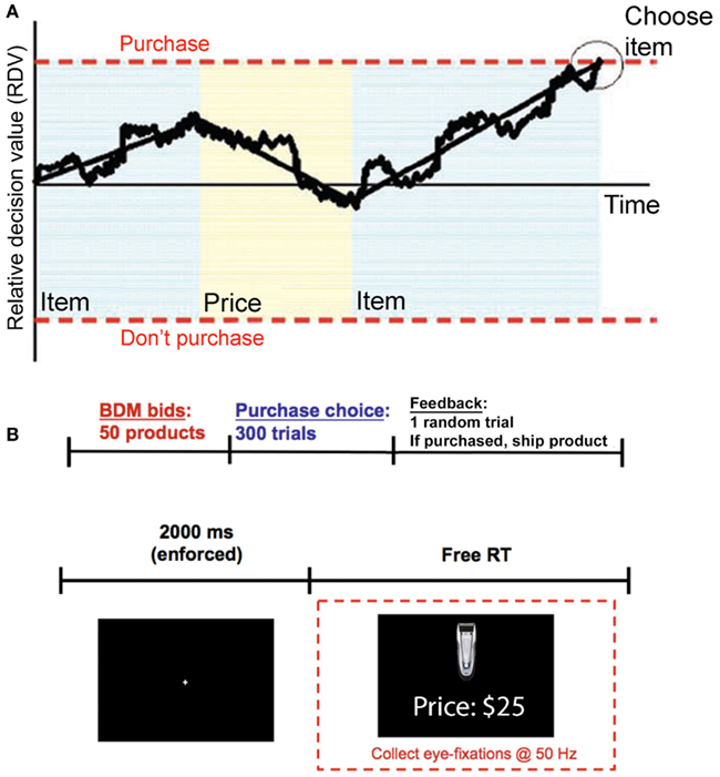
Figure 1. Model and experiment. (A) Model. A relative decision value (RDV) evolves over time with a slope that depends on what the subject is looking at. In addition to the average drift, there is also Gaussian noise. When the RDV reaches one of the two barriers the subject makes the corresponding choice. The shaded regions indicate what the subject is currently looking at, blue for the product and yellow for the price. (B) Timeline. (Top) Subjects first reveal how much they are willing to pay for each of the 50 products, using a BDM auction. Then subjects make 300 purchasing choices (the 50 products at six different prices). At the end of the experiment one trial from the combined tasks is randomly chosen and the subject is paid and/or is shipped the chosen product. (Bottom) Within a choice trial, subjects must first fixate at the center of the screen for 2 s. They are then presented with an item and a price and given unlimited self-paced time to decide whether to buy the item at that price.
A critical feature of the aDDM is that the mean rate of change (drift rate) of the RDV depends on the fixation location at that instant in time (as illustrated in Figure 1A). In particular, when the subject is looking at the item, the evolution of the RDV is given by
and when he is looking at the price, it is given by
where Vt is the value of the RDV at time t within the decision trial, v denotes the subject’s value for the product being considered for purchase, p denotes the price of the purchase, d is a constant controlling the speed of integration (in units of $−1ms−1), θ between 0 and 1 is a parameter reflecting the bias toward the fixated option, and ε is white Gaussian noise with variance σ2 (randomly sampled once every ms). Note that at any point in a trial the RDV is evolving according to one of these two drift rates, depending on where the subject is looking. When the subject shifts his gaze to the other option, the RDV continues to evolve from its current value, but with the other drift rate.
The model assumes that fixations are generated by a stochastic process that is independent of the value of the path that the RDV takes during the trial. Note that this does not rule out the possibility that the fixation process could be affected by the latent value of the product or by the price. In fact, as is described in the methods section below, all of our analyses assume that fixation locations and durations are drawn from the observed empirical distribution, and that the integration process within each fixation continues until the end of the fixation, in which case another fixation is drawn, or until a barrier is crossed, in which case the trial ends. This approach allows us to investigate the comparator process in detail, while taking the fixation process as exogenously given.
Several features of the model are worth highlighting. First, the model has three free parameters: the bias parameter θ, the slope parameter d, and the noise parameter σ. As discussed below and in our previous work (Krajbich et al., 2010; Krajbich and Rangel, 2011) changes in the value of these parameters have important qualitative and quantitative implications for the accuracy and speed of choice. Second, the variables v and p reflect properties of the stimuli being considered, and thus are not parameters of the decision process. In particular, the experimental design described below allows us to measure v and p for each subject and trial independently of the actual purchase decisions, and this information is used to estimate the free parameters of the aDDM. Third, the model includes the standard DDM, in which fixations do not matter, as a special case when θ = 1 (Ratcliff and McKoon, 2008; Milosavljevic et al., 2010). Fourth, the model is almost identical to the one that we have previously proposed for binary choice (Krajbich et al., 2010), except for a slight change in the nature of the stimuli and responses. In particular, in our previous work subjects were shown pictures of two food items, one of the left and one on the right, and they had to choose one of them with a button press. In contrast, here subjects were shown a more complex screen consisting of a picture of an item and a price, and had to indicate with a button press whether they wanted to buy the item at that price. Fifth, when θ < 1 the model predicts that random fluctuations in fixations affect choices. In particular, items are more likely to be purchased when subjects fixate more on the product relative to the price, and less likely to be bought when they fixate relatively more on the price. The intuition is simple and can be easily seen from the two equations above. During fixations on the item, the RDV evolves with an average rate that underestimates the size of the price, which entails a temporary overestimation of the net value, and makes it more likely that the “purchase barrier” is reached. The opposite is true during price fixations.
Materials and Methods
Subjects
Thirty Caltech students participated in the experiment. Subjects received $50 for their participation, which they either kept or used to purchase items using the task described below. Caltech’s Human Subjects Internal Review Board approved the experiment. Subjects provided informed consent prior to their participation.
Task
At the beginning of the experiment subjects were endowed with $50 that they could use to purchase items in two subsequent tasks: a bidding task followed by a purchasing task. The subjects were told that at the end of the experiment one trial from the whole experiment would be randomly selected and implemented. Subjects kept whatever funds they did not spend.
Every subject performed two different tasks in the same order. First, they carried out a bidding task designed to measure the values (i.e., the v in the model) for each product. Second, they carried out a purchasing task that provides the data used to test the aDDM.
In the bidding task, subjects placed bids for the right to purchase 50 different consumer goods including mostly consumer electronics and household items. The task followed the rules of a Becker–Degroot–Marshak (BDM) auction, which is a tool widely used in economics to incentivize subjects to reveal their true values for products (Becker et al., 1964). In brief, a subject is asked to state their willingness-to-pay (WTP) for each of the products. If one of these trials is randomly selected to count, then the experimenter generates a random selling price (from a known uniform distribution from $0 to $50). If the random selling price is less than or equal to the subject’s stated WTP, then the subject purchases the product at the random price and keeps the rest of the $50. If the selling price is greater than the subject’s WTP, then the subject does not purchase the product and keeps the entire $50. Note that the subject cannot influence the price that they pay for the product. They can only indicate whether they would be willing to buy at different prices. Thus, their unique best strategy is to state their true WTP. The order of item presentation was randomized for each subject. Each trial, subjects had unlimited time to examine a high-resolution photograph of the item along with a brief written description of the product on the computer screen and then submit a WTP from $0 to $50 by typing their bid.
The purchasing task is depicted in Figure 1B. Every trial subjects decided whether to buy the shown item at the stated price, or to keep their entire $50. On half of the trials the product was displayed on the top half of the screen with the price on the bottom half of the screen, while on the other half of the trials the locations were switched. Subjects had unlimited time to fixate back and forth between the product and price before indicating their choice to purchase (left arrow) or not purchase (right arrow). All 50 items were randomly presented six times, each time coupled with one of the following six prices: $3, $10, $18, $25, $33, $40. These prices were selected based on piloting data to span the mean WTPs for most items.
At the end of the experiment if one of these trials was randomly selected, then the subject was entitled to receive the product for that trial, and if purchased, we immediately ordered and mailed the product to the subject. The remaining money (up to $50) was immediately paid to the subject in cash.
Eye-Tracking
Subjects’ eye movements were recorded at 50 Hz using a Tobii desktop-mounted eye-tracker. Before each choice trial subjects were required to maintain a fixation at the center of the screen for 2 s before the stimuli would appear. This ensured that subjects began every trial fixating on the same location.
The eye-tracking data were preprocessed using the same procedure as in our previous work (Krajbich et al., 2010; Krajbich and Rangel, 2011). In particular, square regions of interest (ROI) were constructed around the product and price. A fixation was defined as the time from when at least one eye entered the ROI to the moment when both eyes left the ROI. For all measurements following the first fixation and preceding the last fixation of the trial, non-ROI fixations were dealt with according to the following rules:
(1) If the non-ROI fixations were recorded between fixations on the same ROI, then those non-ROI fixations were changed to that ROI. So for example a fixation pattern of “Product,” “Blank,” “Product” would become “Product,” “Product,” “Product.” These non-ROI fixations are typically very short and are likely due to blinks.
(2) If the blank fixations were recorded between fixations on different ROIs, then those blank fixations were recorded as non-decision time and discarded from further analysis. Again, these non-ROI fixations are typically just one eye-tracker measurement (20 ms) and due to transitions between ROIs.
Data Cleaning
Two types of trials were excluded from further analysis. First, for every subject, we excluded trials with items that received a bid of exactly $0 in the first task. These trials are problematic because there are an unusually large number of them (29%) compared to items with small but positive values ($1, $2, $3, etc.) which suggests that these items are being treated differently by the subjects. This could be the case, for example, if these are items that they already own and thus are not seriously considering purchasing. In this case such items could not be used to study the aDDM since they do not involve purchasing decisions. Nevertheless, including these trials does not qualitatively change any of the results.
Second, trials with a net value smaller than −$20, or larger than $20, were also excluded (an additional 28% of trials). These choices are extremely easy for the subjects and so not of particular interest to us. It is only in the −$20 to $20 range that choices are difficult and the aDDM makes interesting predictions. Beyond these net values, subjects are close to 100% accurate and the choice probabilities and reaction times asymptote. Because we were not interested in modeling these very easy choices, we designed the task to minimize trials in this range and so the data in these regions look noisy (due to missing observations) and uninteresting. Additionally, the bins outside this range are scarcely populated, which interferes with our ability to estimate the aDDM accurately.
In principle, this issue could have been avoided through experimental design by choosing prices in the purchasing task close to the values reported in the BDM task. Unfortunately, this is not a feasible solution, because it invalidates the incentive compatibility of the BDM procedure: subjects would have an incentive to bid low amounts in order to ensure low prices in the purchasing task.
Model Simulations and Fitting
The model was fit to the choice and reaction time data using only the even numbered trials of the pooled data set from all the subjects. We then tested the quality of the model fit and predictions by simulating the model using the fitted parameters, and comparing them with the actual data from the odd trials. Thus, the predictions of the model are tested quantitatively and out-of-sample.
The model was fit using a maximum likelihood estimation (MLE) procedure implemented in several steps. First, we ran 3000 simulations for each combination of the model parameters in the grid described below, the six different prices, and the product values (sampled in $2 increments from $0 to $50). In the simulations we randomly sampled fixation times from the empirical distribution conditional on their fixation type (product or price). First-fixation price fixations were sampled separately from the rest of the price fixations because they are statistically shorter than non-first price fixations. Item fixations were sampled conditional on their fixation number (1, 2, 3, 4, 5, 6, 7, or later), and binned on the absolute net value (|v − p|, in $4 increments). We also used the empirical fact that subjects looked at the item first 53.3% of the time. We also took account of the latency for the first fixation, as well as for the transition time between fixations. We did this by computing the difference between the average reaction time and the average total fixation time (time spent looking at either the product or the price), and adding this trial-independent estimate to the simulated reaction times. This average “non-decision” time was 336 ms, consistent with non-decision times in our previous work (355 ms in Krajbich et al., 2010) and in other DDM studies of binary choice (365 ms in Milosavljevic et al., 2010 and 338 ms in Ratcliff, 2002, for example).
Second, we computed the probability of each observation in the data, for each set of parameters, as follows. The empirical spread of reaction times ranged from 495 ms to 47.1 s so in the fitting procedure we discarded any simulation trials below 400 ms or above 48 s. The rest of the reaction times were separated into bins of 400 ms except for the final bin, which went from 4800 ms to 48 s. For each net value bin ($4 increments), we split the data into buy and no-buy trials, then for each group counted the number of data trials in each reaction time bin, and similarly calculated the probability of a simulation trial occurring in each reaction time bin. Note that the first two steps are necessary to compute the likelihood function of the data because there is no known closed-form solution for the aDDM.
Third, we identified the set of parameters that maximized the log-likelihood of the data by taking the logarithms of each of these probabilities and summing them up. The resulting number is used to assess how well the model fit the data, with larger numbers (closer to zero) indicating better fits. The search was performed over a grid of values for d, σ, and θ. The MLE search was carried out in two steps. First we searched over a coarse grid with d in (0.00006, 0.000065, 0.00007), σ in (0.0228, 0.0237, 0.0247), and θ in (0.7, 0.8, 0.9, 0.99). Second, we used the results from the first search to define a narrower search with d in (0.00006, 0.000065), σ in (0.0218, 0.0228, 0.0237), and θ in (0.5, 0.6, 0.7, 0.8). The initial parameters were chosen based on comparisons to our previous results (Krajbich et al., 2010). The best-fitting parameters at this stage were d = 0.000065, σ = 0.02275, and θ = 0.7.
The previous procedure assumes that there is no motor latency, namely that the subject enters his choice instantaneously once the RDV crosses a barrier. To address this problem, we carried out the following additional step in the model fitting process. We simulated the model with the best MLE parameters described above, and then compared the average duration of the final fixations with those from the actual data. Note that this comparison is important because, to the extent that subjects maintain fixation during the motor latency period, our measured durations for final fixations include the actual duration of the fixation and the motor latency. Consistent with this concern, our predicted final fixation durations were on average 73 ms shorter than actual measured fixations. Taking this value as the mean motor latency, we redid the model fitting procedure with the added feature that there is a 73 ms delay after the decision is made. As before, we began with a coarse grid search, this time with d in (0.00006, 0.000065, 0.00007), σ in (0.0228, 0.0237, 0.0247), and θ in (0.6, 0.7, 0.8, 0.9). Second, we used the results from the first search to define a narrower search with d in (0.000065), σ in (0.0218, 0.0228, 0.0233, 0.0237), and θ in (0.6, 0.65, 0.7, 0.75, 0.8, 0.9). The reported model fits below include the motor latency correction, which is also used in all simulations reported in the paper.
Goodness-of-Fit Calculations
For Figures 2B,C, and 5 we could not compute χ2 goodness-of-fit statistics because the dependent variables are not binary. Instead we devised the following alternative goodness-of-fit statistic: (1) for each bin of the independent variable we “correct” the dependent variable by subtracting the average simulated value from each subject’s average value. (2) We then run a weighted least-squares (WLS) regression with the “corrected” dependent variable. The weights in the regression are equal to the inverse of the variance. Note that if the simulations fit the data well, then the “corrected” data should be a flat line at 0. On the other hand, if the simulation fits poorly, then the WLS coefficients should be non-zero. So, for goodness-of-fits, we report the p-values for the coefficients of these WLS regressions. If the p-values are less than 0.05 then we reject that the model accurately fits the data.
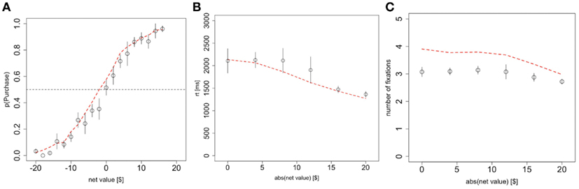
Figure 2. Basic psychometrics. (A) Probability of purchasing the product as a function of the net value (product value – price). (B) Reaction times as a function of the magnitude of the net value. (C) The number of fixations in a trial, as a function of the magnitude of the net value. Black circles indicate data from the odd-numbered trials of the subject data, and red dashed lines indicate the simulated data from the aDDM. Bars are standard error bars, clustered by subject.
Results
Model Fit
We fitted the model to the even numbered trials from the group data using MLE. The model has three free parameters: the constant determining the speed of integration d, the discount parameter θ, and the noise parameter σ. The model was fit under the assumption that time evolves in 1 ms discrete steps. We selected the parameters that maximized the probability of the observed choices and reaction times, conditional on the net value of the offer (see Materials and Methods for details). The best-fitting model had parameters d = 0.000065 $−1ms−1, σ = 0.0233, and θ = 0.7.
For comparison purposes, in our previous work on binary and trinary choice we found that the parameters d = 0.0002 ms−1, σ = 0.02, and θ = 0.3 provided the best fit for the data (Krajbich et al., 2010; Krajbich and Rangel, 2011). Since these parameters were fitted using methods very similar to those used here, their comparison provides some insight about the computational differences between binary choices and yes-no purchasing decisions. Consider some of the most salient relationships. First, we found that the noise parameter σ was nearly identical in the two cases, which suggests a similar amount of computational noise in both problems. Second, we found that the slope parameter d was about 1/3 smaller in the current data set. This difference needs to be interpreted with caution, however, because the slope depends on the scale with which values are measured. In particular, multiplying the net values by a constant a results in a new fit that decreases d by a factor of 1/a, and leaves the fits of the other two parameters unchanged. The difference is then easily explained by the fact that values in our previous paper were measured using liking-rating differences that ranged from −5 to +5, whereas here the value differences ranged from −20 to +20. Third, the bias is significantly smaller than in our previous work: θ = 0.7 vs. θ = 0.3 previously (recall that θ = 1 is the case of no bias, so that as theta increases from 0 to 1 the size of the bias goes down). Nevertheless, as we will see in more detail below, with θ = 0.7 there is still a non-trivial effect of visual fixations on the choice process.
Model Simulation
In order to investigate the ability of the model to predict the data quantitatively, we then simulated the model 10,000 times per value and price combination (binning values every $2), using the estimated maximum likelihood parameters, and by sampling fixation lengths from the actual empirical fixation data (see Materials and Methods for details). Throughout, we assume that fixations always alternate between the product and price, and that the location of the first fixation is chosen probabilistically to match the empirical data (look at the product first with probability 53.3%). The results of the simulations are described below.
Note that all comparisons of the model to the data were made out-of-sample using only on the odd-numbered trials, since the model was fitted to the even-numbered trials. Also, in all of the figures below red curves represent the simulations, and black symbols and curves represent the data.
Unless otherwise noted, throughout the results, goodness-of-fit p-values are based on two-sided t-tests of the regression parameters against zero (see Materials and Methods for goodness-of-fit details), and p-values for trends in the subject data are based on two-sided t-tests of the mixed-effects regression parameters against zero. Each mixed-effects regression contains random effects for the intercept and all other regressors.
Basic Psychometrics
In this section we investigate how well the aDDM predicted the choice and reaction time data on the half of the data that it was not fitted to, and additionally estimate the effects of choice difficulty on average reaction times and number of fixations. Our measure of choice difficulty is the absolute (unsigned) net value, which tells us the difference in value between the item and the price. With this measure, the hardest decision is one where the item value and price are identical, leading to a net value of $0.
The fitted model accounted for the choice and reaction time curves well. Choices were a logistic function of net value in both the data and the simulations (Figure 2A; χ2 goodness-of-fit: p = 0.8). As expected, subjects were more likely to purchase on trials with a positive net value and less likely to purchase on trials with a negative net value.
Reaction times significantly increased with difficulty at an average rate of 42 ms/$ (p < 10−10 mixed-effects) and the aDDM also provided a close fit to the data (Figure 2B; goodness-of-fit slope: p = 0.9, intercept: p = 0.7).
The average number of fixations in a trial exhibits a small but significant (p < 10−5 mixed-effects) response to increasing difficulty at a rate of 0.016 fixations/$, though the aDDM does not fit as well here (Figure 2C; goodness-of-fit slope: p = 0.0005, intercept: p = 10−13). Even after correcting for the difference in scale, the size of effect is about 1/3 of the one that we previously observed with choices between food items (Krajbich et al., 2010).
As shown in Figure 2C, the model systematically predicts 0.7 excess fixations. This mismatch has been consistently observed with the aDDM (Krajbich et al., 2010; Krajbich and Rangel, 2011), is an unavoidable consequence of the procedures used to carry out the simulations, and does not reflect an inherent limitation of the model. In fact, this bias is present even if one simulates a dataset using the aDDM, and then carries out the model fitting exercise on the simulated data. More concretely, the problem is due to the fact that we have to sample fixations from the empirical distribution of non-final fixations, but many of those fixations are cut short by a barrier crossing and become final fixations in the simulations. The longer the fixation, the more likely it is to cross a barrier, and so the average middle fixation duration is shorter in the simulations; this means that more fixations are required to achieve the same reaction times in our simulations as in the actual data. Nevertheless, the mismatch is larger here than previously observed and the aDDM also over-estimates the effect of difficulty on the number of fixations, though the difference is quite small (0.03 fixations/$).
Model Predictions and Choice Biases
The model with θ = 0.7 makes several stark predictions about the relationship between fixations, choices, and reaction times that we test using the eye-tracking data.
First, the model predicts that the last fixation of the trial is more likely to be to the product when the subject decides to purchase it, unless the BDM value of the item is sufficiently smaller than the price. It also predicts that the last fixation is likely to be to the price when the subject decides not to purchase the item, unless the price is sufficiently lower than the value of the product. To see the intuition for this effect, consider the case in which the last fixation is to the product. In this case, the RDV tends to climb toward the purchase barrier, unless the value of the item is smaller than θ *p. Figure 3A looks at the probability that the last fixation is to the chosen item (product = purchase or price = no purchase) as a function of the difference in value between the last-seen stimulus and the other stimulus. The figure shows that a small but noticeable bias of this type is present in both the data and the simulations (χ2 goodness-of-fit: p = 0.4).
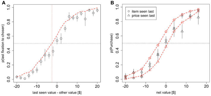
Figure 3. Model predictions and results. (A) The probability that the last fixation of the trial is to the chosen stimulus (product or money) as a function of the difference in value between the last-seen stimulus and the other stimulus. (B) The probability of purchasing the item as a function of net value, contingent on whether the last fixation was to the product or to the price. Black circles indicate data from the odd-numbered trials of the subject data, and red dashed lines indicate the simulated data from the aDDM. Bars are standard error bars, clustered by subject.
For an additional test of the prediction that there is an overall bias toward choosing the item that is looked at last, we ran a logit regression using the entire dataset and variables in Figure 3A to test whether the intercept was greater than 0. The logit confirmed that indeed the intercept was greater than 0 (p = 0.03 based on a one-sided t-test on the entire dataset), indicating that for a net value of $0, the probability of choosing the item that is looked at last is significantly greater than 0.5. We also ran an additional version of this analysis with a different logit regression for each subject and found that the average intercept was marginally significantly greater than zero (p = 0.07 one-sided t-test), providing further evidence for this effect.
Second, the model predicts that the choice curves should be different for trials where the last fixation was to the product or to the price. Specifically, it predicts that subjects should be more likely to purchase the item if the last fixation was to the product than if it was to the price. This follows directly from the fact that with θ < 1, the net value of the trade is overestimated when fixating on the product, and underestimated when fixating on the price. This effect is small but noticeable in both the simulations and the data (Figure 3B; χ2 goodness-of-fit item seen last: p = 0.01, price seen last: p = 0.3). To test the significance of this effect in the data, we ran two logistic regressions on the entire dataset and variables from Figure 3B, one for trials where the product was seen last and one for trials where the price was seen last. For trials where the product was seen last the logit intercept was significantly greater than zero (p = 0.03 one-sided t-test) while for trials where the price was seen last the logit intercept was significantly less than zero (p = 0.05 one-sided t-test). Subject-level analyses were inconclusive (p = 0.53), likely due to many cases of perfect separation and small numbers of observations for other subjects in some of the bins.
Third, the model predicts that more time spent looking at the product over the course of the trial will bias subjects toward purchasing the good, and that is what we see in the data (Figure 4A; χ2 goodness-of-fit: p = 0.4). Here the total fixation time advantage for the item is just the total amount of time spent looking at the item minus the total amount of time spent looking at the price, in that trial. One important concern with this result has to do with the exogeneity of the fixation lengths. In particular, it could be that the choice bias shown in Figure 4A is due to a positive relationship between the total fixation time advantage for the item and the net value. To address this concern we ran a mixed-effects logit regression including net value and total fixation time advantage for the item as independent variables and purchasing as the dependent variable. The effect of the total fixation time advantage was highly significant (p < 10−6), ruling out this alternative explanation. Furthermore, a regression of the total fixation time advantage for the item on net value shows no significant relationship (5.2 ms/$, p = 0.09 mixed-effects linear regression, two-sided t-test).
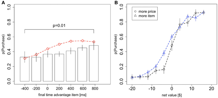
Figure 4. Choice biases. (A) The probability of purchasing the item as a function of the difference in total fixation time (over the whole trial) between the product and the price. Black circles indicate data from the odd-numbered trials of the subject data, and the red dashed line indicates the simulated data from the aDDM. The p-value is from a one-sided t-test. (B) The probability that the product is chosen as a function of the net value, conditional on whether more time was spent looking at the product or the price in that trial. Bars are standard error bars, clustered by subject.
An alternative way to investigate this effect is to split trials based on whether the subject spent more time looking at the product or the price. As expected, controlling for net value, subjects were more likely to purchase the product if they spent more time looking at it than if they spent more time looking at the price (Figure 4B). To test for a significant difference between these curves, we ran two logistic regressions (analogous to the analysis for Figure 3B) on the entire dataset and variables in Figure 4B, one for trials where the product was looked at more and one for trials where the price was looked at more. For trials where the subjects looked longer at the product, the logit intercept was significantly greater than zero (p < 0.01 one-sided t-test) while for trials where the subjects looked longer at the price, the logit intercept was significantly less than zero (p = 0.02 one-sided t-test). As a further test, we ran identical subject-level logits and again found a significant difference between the intercepts for trials where the product was looked at more and the intercepts for trials where the price was looked at more (p = 0.03, one-sided paired t-test; 10 subjects were excluded due to perfect separation).
Finally, the model also predicts a precise quantitative relationship between reaction times and net values, as a function of the type of decision made. As shown in Figure 5, the model provides a fairly good description of the associated patterns (Figure 5A goodness-of-fit slope: p = 0.5, intercept: p = 0.8; Figure 5B goodness-of-fit slope: p = 0.11, intercept: p = 0.12). The intuition behind these patterns goes as follows. In this experiment, we can define a mistake as either a trial where the subject purchased an item with a negative net value or a trial where the subject didn’t purchase an item with a positive net value. With θ < 1, mistakes tend to occur when the subject has spent more time looking at the worse option. Therefore, mistakes take longer than correct choices because the average drift rate when the subject is looking at the worse item is always smaller than when the subject is looking at the better item, and a smaller drift rate requires more time for the RDV to reach the choice barrier. Furthermore, the bigger the mistake, the longer the decision should take, up to a point. There is a counteracting force, which is that big mistakes shouldn’t happen and so if the subject takes some time to make his decision then he won’t make these big mistakes. In other words, given a reasonable amount of time, the overwhelming average drift rate in favor of the correct option should overwhelm the noise in the decision process. Therefore, big mistakes must occur due to large spikes in the noise, and these spikes must occur early in the trial before there is overwhelming evidence for the correct choice. Without a formal model it would be unclear at what point these two counteracting forces should shift in power, but our model predicts the trend in the data quite accurately.
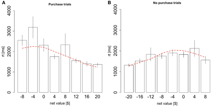
Figure 5. Reaction times conditional on choice. (A) Reaction times as a function of the net value, conditional on purchasing the product. (B) Reaction times as a function of the net value, conditional on not purchasing the product. Black bars indicate data from the odd-numbered trials of the subject data, and the red dashed lines indicate the simulated data from the aDDM. Bars are standard error bars, clustered by subject.
Fixation Properties
Finally, we investigate the extent to which the fixation process resembles the assumptions and predictions of the model. To do so we look at the first fixations of each trial, as well as the “middle fixations” which are any fixations that are not the first fixation or the last fixation of the trial. We treat the last fixations of the trials separately since in the model these fixations are cut short by the choice.
Consistent with previous findings on choice between products, we found no significant correlation between product value and mean fixation duration for either first fixations or middle fixations. There was a small effect of price and a large effect of choice difficulty on middle item mean fixation duration (Figures 6A–C, price: 10 ms/$, p = 0.02, product value: 6.7 ms/$, p = 0.3, net value: −35 ms/$, p < 10−6, two-sided t-tests based on a mixed-effects regression with all three factors). However, we found no such effect for middle price fixations (Figures 6D–F, price: 0.85 ms/$, p = 0.08; product value: −0.018 ms/$, p = 0.98; net value: −1.38 ms/$, p = 0.08, two-sided t-tests based on a mixed-effects regression with all three factors), or for first fixations to either products (price: 0.089 ms/$, p = 0.9; product value: 0.37 ms/$, p = 0.5; net value: −0.9 ms/$, p = 0.2, two-sided t-tests based on a mixed-effects regression with all three factors) or prices (price: 0.11 ms/$, p = 0.8; product value: 0.71 ms/$; p = 0.2, net value: −0.51 ms/$, p = 0.5, two-sided t-tests based on a mixed-effects regression with all three factors).
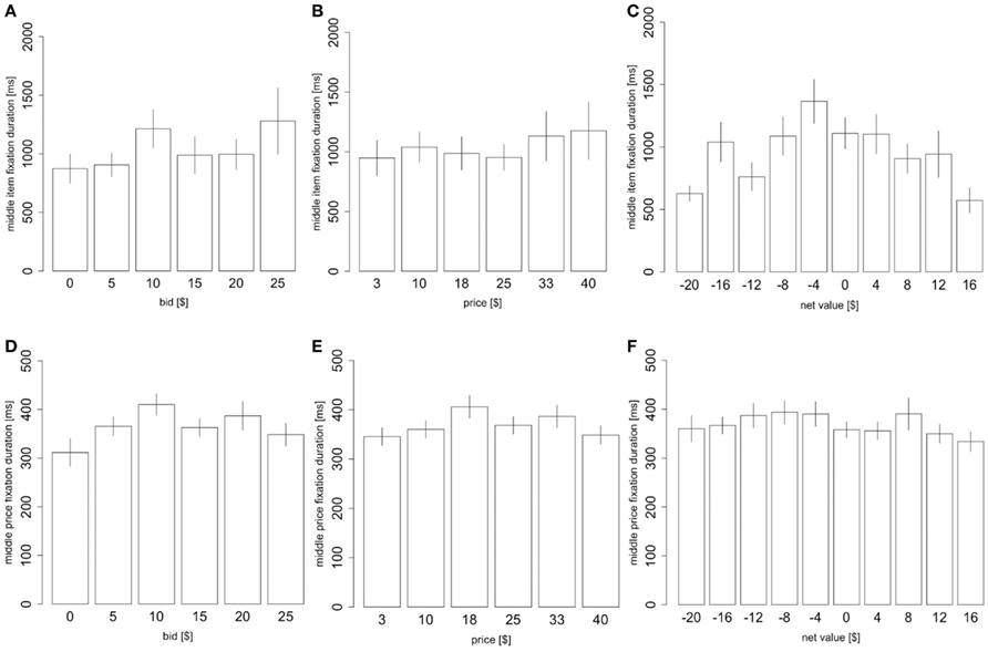
Figure 6. Fixation properties. (A) The duration of middle item fixations as a function of the item value, (B) price, and (C) net value. (D) The duration of middle price fixations as a function of the product value, (E) price, and (F) net value. Bars are standard error bars, clustered by subject.
Consistent with the predictions of the model, and with previous findings (Krajbich et al., 2010; Krajbich and Rangel, 2011), we also found that first and last fixations were significantly shorter than middle fixations both for products (first: p = 10−7, last: p = 0.0001, two-sided paired t-tests) and prices (first: p = 10−5, last: p = 0.03, two-sided paired t-tests; Figure 7A). Our model does not predict the first fixation effect, but we have seen it consistently in all of our previous related studies. The model does predict shorter final fixations, since final fixations are just middle fixations cut short by the RDV crossing a decision barrier.
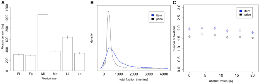
Figure 7. Item vs. price fixations. (A) Fixation duration as a function of fixation type: first fixation to item, first fixation to price, middle fixation to item, middle fixation to price, last fixation to item, and last fixation to price. Note that “first/last fixation” means the first/last fixation of the trial, not the first/last fixation to each stimulus. (B) Density plot of the total trial time spent looking at the item (blue) and price (black). (C) The number of item and price fixations in a trial, as a function of the magnitude of the net value. Bars are standard error bars, clustered by subject.
Figure 7B compares the distribution of price and product total fixation times, i.e., summed over the whole trial. The distribution of total fixation times for items has a larger mean and standard deviation than that for prices (items: M = 1064 ms, SD = 1266 ms; prices: M = 471 ms, SD = 390 ms; M: p = 10−8, SD: p = 10−7; statistics computed first at the individual level, and then compared across individuals using paired t-tests).
Finally, Figure 7C shows the average number of item fixations and price fixations per trial. We see that both types of fixations follow the same trend as seen in the aggregate Figure 2C, but there are consistently about 0.5 fewer price fixations than item fixations. However, this result is not surprising, given that item fixations are longer than price fixations and so are more likely to be the last fixation of the trial. For trials with an even number of fixations there is always an equal number of fixations to item and price, regardless of the last fixation location. But for trials with an odd number of fixations there will always be one more fixation for the last-seen stimulus. Since the last fixation of the trial is to the item in 79% of trials, we indeed expect there to be ∼0.4 fewer price fixations than item fixations.
Discussion
We have described the results of an eye-tracking experiment of purchasing decisions designed to investigate if the aDDM is able to provide a reasonable quantitative description of the relationship between the fixation, choice, and reaction time data in the case of simple purchasing decisions. The motivation for doing this is that in previous work we have found that the model provides a remarkably accurate description of these variables and their interrelationship in the case of binary and trinary food choices (Krajbich et al., 2010; Krajbich and Rangel, 2011). Thus, the research agenda here is to investigate the extent to which the aDDM also applies to other types of decisions, what changes are needed to account for new aspects of the task, and more generally when it breaks down and why.
We find that the model provides a reasonably accurate description of the purchasing decision data, although of significantly lower accuracy than in our previous work. This shows that purchasing decisions introduce new aspects into the problem that are not well captured by the simple aDDM and that need to be investigated in future research (see below for some conjectures). However, we find that the best-fitting aDDM has parameters similar to what we found in our previous work, with the exception of the parameter controlling the magnitude of the visual fixation bias in the value integration process. In particular, the bias parameter went from θ = 0.3 in our previous work to θ = 0.7 in the current dataset, which constitutes a sizable reduction in the size of the fixation-driven choice biases. Nevertheless, many of the key biases predicted by the model were still present in the purchasing data, albeit of a smaller magnitude than those found in the previous studies and generally not as big as the model predicted. Furthermore, once again we found that these effects are not due to subjects looking longer at products (or less at prices) in trials with a high net value.
In judging the reduced accuracy of the model it is important to keep in mind that we are imposing some very strict tests on the model. First, we are fitting the model on one half of the data and then predicting on the other half of the data, rather than merely showing fits to the data. Second, we are fitting the model on only the choice and reaction time curves (Figures 2A,B). It is quite likely that we could have achieved nicer results by fitting to the fixation trends as well (e.g., Figure 4A), but that would detract from a main feature of the model, which is the ability to predict fixation trends using only choice and reaction time data.
These results are important for several reasons.
First, they provide additional evidence that the aDDM provides a reasonably accurate and robust characterization of how the brain computes value-based choices of different types. An important difference with our previous paradigms is that here subjects had to integrate the value of two very different types of stimuli.
Second, the results provide some new insights to the literature on decision field theory (DFT) by Busemeyer and others (Busemeyer and Townsend, 1993; Diederich, 1997, 2003; Roe et al., 2001; Busemeyer and Diederich, 2002; Johnson and Busemeyer, 2005; Tsetsos et al., 2010). See also the closely related models of Usher and McClelland (2004) and Usher et al. (2008). These models have also investigated the impact that random fluctuations in attention have on choice accuracy and reaction time. In particular, although the DFT model has not been previously applied to the type of simple purchasing decisions studied here, it is easily extended to this case. Such an extension highlights an important difference between the two models: DFT assumes that attention (and thus the drift rate) fluctuates continuously across time according to either a stationary or Markov process, while we assume that there are only two states of attention and that the current state is indicated by the subject’s fixation location. This is an important difference because, as a result, although it can account for the basic choice and reaction time profiles, DFT cannot account for many of the fixation patterns described here and in our previous work on multi-option choice (Krajbich et al., 2010; Krajbich and Rangel, 2011).
Our model is closer in spirit to multiattribute decision field theory (MDFT; Diederich, 1997, 2003; Busemeyer and Diederich, 2002) but in that model it is assumed that the attributes are processed in a serial manner, equivalent to the case of θ = 0 in our model. Again, that model cannot account for the trends in our data. For purchasing decisions, our aDDM represents something like a hybrid between DFT and MDFT, with the additional specification that gaze location determines the weights on the attributes. It is also worth noting that analytic solutions have been derived for those models, under certain assumptions about the evolution of the attribute weights.
However, we emphasize that our purpose here is not to rule out these alternative models and explanations, but to argue that the aDDM provides a simpler explanation of value-based decision-making that can quantitatively account for the effects of visual attention on choice in both purchasing and multi-option decisions. Obviously this simplicity comes at a cost: we do not account for possible shifts of attention to positive or negative attributes within a fixation. Instead we assume that evidence for an option is accumulated with an average rate that is proportional to the latent value (i.e., the BDM value), which should reflect the mixture of positive and negative attributes. Shifts of attention to different attributes within a fixation are therefore only taken into account by the Gaussian random noise that is added to the average evidence accumulation.
Second, the results show that the basic mechanisms at work in the aDDM also seem to apply to cases in which one of the options is numeric or symbolic, instead of a more complex visual stimulus. This is important because it provides some new hints about the nature of the processes at work. It has been previously speculated that the process of value integration and comparison is noisy because the brain needs to take repeated noisy samples of the value of the stimuli being evaluated, and that visual attention matters because it guides the sampling process (Busemeyer and Townsend, 1993; Krajbich et al., 2010; Glockner and Herbold, 2011; Krajbich and Rangel, 2011). This is a natural interpretation for stimuli that are visually complex, but it is not obvious if the same holds true for numerical price representations. The results here show that this is indeed the case: although fixations to prices are shorter and less variable, the results suggest that they are also integrated noisily over time. This suggests that the process of noisy dynamic integration of value might be a widespread aspect of the choice process, and not just applicable to complex visual stimuli.
To lend further support to this claim, we carried out model fittings of an additional model that allows for different values of the visual fixation bias parameter θ, depending on whether the product or the price is being fixated on. We found that adding this additional parameter did indeed significantly improve the fit of the model, but that the best fitted θ for the item was still 0.7, and the best fitted theta for the price θ changed only slightly to 0.6. This provides further support for the finding that the integration processes for the product and price information have similar properties.
Third, the difference between the magnitude of the visual biases raises the following interesting puzzle: why is it the case then that the visual bias for the products during the purchasing decisions is much lower than the bias for the foods during binary choice? After all, the complexity of the pictures used to display the products here is very similar to that of the food pictures used in our previous work. One potential but speculative explanation is that there is a visual difference in the two displays. During binary choice two similar food pictures are displayed, while two different types of visual images – a visually complex food picture and a simple number – are displayed during purchasing decisions. Looking at one picture might inhibit working memory for the other picture (including low-level rehearsal captured by θ) more strongly than looking at a number, and vice-versa (Baddeley, 2003). The reduced inhibition in the picture-number paper would be manifested by a higher value of θ, just as we infer from the data. If this hypothesis is correct, then when prices are presented in a complex visual display (e.g., stacks of money and coins) rather than as a simple number, we might expect a θ lower than what was measured in this task.
Fourth, the fact that price fixations were shorter and less variable than those for products is consistent with the idea that the deployment of visual attention is based on the utility of information (Gottlieb and Balan, 2010). An important open question for future work is to develop and test a full optimal model of visual attention deployment. Note that this imposes more stringent restrictions on the fixation process than just having shorter fixations on stimuli that are easier to process, or having less noise associated with them. One place where the aDDM was noticeably inaccurate was in the prediction of how the number of fixations varies with choice difficulty, and so clearly we need a better understanding of how fixations work in purchasing decisions.
Fifth, the results have obvious implications for marketing and public policy. In particular, they show that sellers may be able to use strategic product and price placement, as well as manipulation of saliency (Milosavljevic et al., 2012), to encourage consumers to purchase their products. Also, sellers of inferior products may benefit from deliberately putting people under unnaturally high time pressure (Diederich, 1997). In the aDDM, time pressure creates a large rate of “mistakes” (choices with a negative net value) that decreases in longer trials. Indeed, some high-pressure phone and door-to-door sales tactics could be construed as attempts to bring a premature halt to a slow DDM process, in order to create large consumer mistakes that benefit the sellers. The aDDM approach gives a new way to study this process scientifically and can suggest policy remedies (e.g., “cooling off periods,” during which buyers can costlessly renege on an agreement to sell; Camerer et al., 2003).
Of course such manipulations have their limits. Compared to previous results with multi-option choice, the effects of visual attention are quite reduced in our purchasing task. Therefore, if the product under consideration is substantially worse than its price then the drift rate will always tend toward the “do not buy” threshold, regardless of what the subject is looking at. In addition, noticeable attention manipulations such as forcing the subject to look at a product for a long time may alert the subject and alter the decision-making process. Nevertheless, previous research has shown that it is indeed possible to influence choices by exogenously manipulating fixation times (Shimojo et al., 2003; Armel et al., 2008), consistent with the idea that visual fixations are influencing the choices and not vice-versa.
Finally, the study provides additional evidence of the value of utilizing eye-tracking data in conjunction with carefully designed decision tasks to test process models of decision-making. In this sense, it builds on the seminal pioneering work of Johnson and colleagues (Johnson et al., 1988, 2002, 2007; Camerer and Johnson, 2004), as well as more recent applications (Russo et al., 2006, 2008; Raab and Johnson, 2007; Horstmann et al., 2009; Glockner and Herbold, 2011; Russo and Yong, 2011; Glockner et al., 2012). For an outstanding recent review, see Russo (2010).
Conflict of Interest Statement
The authors declare that the research was conducted in the absence of any commercial or financial relationships that could be construed as a potential conflict of interest.
Acknowledgments
This research was supported by grants to Antonio Rangel from the NSF (SES-0851408, SES-0926544, SES-0850840), NIH (R01 AA018736), and Lipper Foundation. Ian Krajbich was supported by a National Science Foundation Integrative Graduate Education and Research Traineeship. Dingchao Lu was supported by a Summer Undergraduate Research Fellowship from the California Institute of Technology.
References
Armel, K. C., Beaumel, A., and Rangel, A. (2008). Biasing simple choices by manipulating relative visual attention. Judgm. Decis. Mak. 3, 396–403.
Baddeley, A. (2003). Working memory: looking back and looking forward. Nat. Rev. Neurosci. 4, 829–839.
Basten, U., Biele, G., Heekeren, H., and Fieback, C. J. (2010). How the brain integrates costs and benefits during decision making. Proc. Natl. Acad. Sci. U.S.A. 107, 21767–21772.
Becker, G. M., Degroot, M. H., and Marschak, J. (1964). Measuring utility by a single-response sequential method. Behav. Sci. 9, 226–232.
Bogacz, R. (2007). Optimal decision-making theories: linking neurobiology with behaviour. Trends Cogn. Sci. (Regul. Ed.) 11, 118–125.
Busemeyer, J. R., and Diederich, A. (2002). Survey of decision field theory. Math. Soc. Sci. 43, 345–370.
Busemeyer, J. R., and Johnson, J. G. (2004). “Computational models of decision making,” in Blackwell Handbook of Judgment and Decision Making, eds D. J. Koehler and N. Harvey (Malden, MA: Blackwell Publishing Ltd), 133–154.
Busemeyer, J. R., and Rapoport, A. (1988). Psychological models of deferred decision making. J. Math. Psychol. 32, 91–134.
Busemeyer, J. R., and Townsend, J. T. (1993). Decision field theory: a dynamic-cognitive approach to decision making in an uncertain environment. Psychol. Rev. 100, 432–459.
Camerer, C., Issacharoff, S., Loewenstein, G., O’Donoghue, T., and Rabin, M. (2003). Regulation for conservatives: behavioral economics and the case for “asymmetric paternalism.” Univ. PA. Law Rev. 151, 1211–1254.
Camerer, C., and Johnson, E. J. (2004). “Thinking about attention in games: backward and forward induction,” in The Psychology of Economic Decisions, eds J. Carillo and I. Brocas (New York: Oxford University Press), 111–129.
Diederich, A. (1997). Dynamic stochastic models for decision making under time constraints. J. Math. Psychol. 41, 260–274.
Diederich, A. (2003). MDFT account of decision making under time pressure. Psychon. Bull. Rev. 10, 157–166.
Glockner, A., Heinen, T., Johnson, J. G., and Raab, M. (2012). Network approaches for expert decisions in sports. Hum. Mov. Sci. 31, 318–333.
Glockner, A., and Herbold, A.-K. (2011). An eye-tracking study on information processing in risky decisions: evidence for compensatory strategies based on automatic processes. J. Behav. Decis. Mak. 24, 71–98.
Gold, J. I., and Shadlen, M. N. (2007). The neural basis of decision making. Annu. Rev. Neurosci. 30, 535–574.
Gottlieb, J., and Balan, P. (2010). Attention as a decision in information space. Trends Cogn. Sci. (Regul. Ed.) 14, 240–248.
Hare, T., and Rangel, A. (2010). Neural computations associated with goal-directed choice. Curr. Opin. Neurobiol. 20, 262–270.
Hare, T., Schultz, W., Camerer, C., O’Doherty, J. P., and Rangel, A. (2011). Transformation of stimulus value signals into motor commands during simple choice. Proc. Natl. Acad. Sci. U.S.A. 108, 18120–18125.
Horstmann, N., Ahlgrimm, A., and Glockner, A. (2009). How distinct are intuition and deliberation? An eye-tracking analysis of instruction-induced decision modes. Judgm. Decis. Mak. 4, 335–354.
Johnson, E. J., Camerer, C., Sen, S., and Rymon, T. (2002). Detecting failures of backward induction: monitoring information search in sequential bargaining. J. Econ. Theory 104, 16–47.
Johnson, E. J., Haubl, G., and Keinan, A. (2007). Aspects of endowment: a query theory of value construction. J. Exp. Psychol. Learn. Mem. Cogn. 33, 461–474.
Johnson, E. J., Payne, J. W., and Bettman, J. R. (1988). Information displays and preference reversals. Organ. Behav. Hum. Decis. Process 42, 1–21.
Johnson, J. G., and Busemeyer, J. R. (2005). A dynamic, stochastic, computational model of preference reversal phenomena. Psychol. Rev. 112, 841–861.
Kable, J., and Glimcher, P. (2009). The neurobiology of decision: consensus and controversy. Neuron 63, 733–745.
Krajbich, I., Armel, K. C., and Rangel, A. (2010). Visual fixations and the computation and comparison of value in simple choice. Nat. Neurosci. 13, 1292–1298.
Krajbich, I., and Rangel, A. (2011). Multialternative drift-diffusion model predicts the relationship between visual fixations and choice in value-based decisions. Proc. Natl. Acad. Sci. U.S.A. 108, 13852–13857.
Leite, F. P., and Ratcliff, R. (2010). Modeling reaction time and accuracy of multiple-alternative decisions. Atten. Percept. Psychophys. 72, 246–273.
Milosavljevic, M., Malmaud, J., Huth, A., Koch, C., and Rangel, A. (2010). The drift diffusion model can account for the accuracy and reaction time of value-based choices under high and low time pressure. Judgm. Decis. Mak. 5, 437–449.
Milosavljevic, M., Navalpakkam, V., Koch, C., and Rangel, A. (2012). Relative visual saliency differences induce sizable bias in consumer choice. J. Consum. Psychol. 22, 67–74.
Philiastides, M., Biele, G., and Heekeren, H. (2010). A mechanistic account of value computation in the human brain. Proc. Natl. Acad. Sci. U.S.A. 107, 9430–9435.
Raab, M., and Johnson, J. G. (2007). Expertise-based differences in search and option-generation strategies. J. Exp. Psychol. Appl. 13, 158–170.
Rangel, A., Camerer, C., and Montague, P. R. (2008). A framework for studying the neurobiology of value-based decision making. Nat. Rev. Neurosci. 9, 545–556.
Ratcliff, R. (2002). A diffusion model account of response time and accuracy in a brightness discrimination task: fitting real data and failing to fit fake but plausible data. Psychon. Bull. Rev. 9, 278–291.
Ratcliff, R., and McKoon, G. (1997). A counter model for implicit priming in perceptual word identification. Psychol. Rev. 104, 319–343.
Ratcliff, R., and McKoon, G. (2008). The diffusion model: theory and data for two-choice decision tasks. Neural Comput. 20, 873–922.
Ratcliff, R., and Rouder, J. N. (2000). A diffusion model account of masking in two-choice letter identification. J. Exp. Psychol. Hum. Percept. Perform. 26, 127–140.
Ratcliff, R., and Smith, P. (2004). A comparison of sequential sampling models for two-choice reaction time. Psychol. Rev. 111, 333–367.
Roe, R. M., Busemeyer, J. R., and Townsend, J. T. (2001). Multialternative decision field theory: a dynamic connectionist model of decision making. Psychol. Rev. 108, 370–392.
Rushworth, M. F. S., Noonan, M. P., Boorman, E. D., Walton, M. E., and Behrens, T. E. (2011). Frontal cortex and reward-guided learning and decision-making. Neuron 70, 1054–1069.
Russo, J. E. (2010). “Eye fixation as a process trace,” in A Handbook of Process Tracing Methods for Decision Research, eds M. Schulte-Mecklenbeck, A. Kuehberger, and R. Ranyard (New York: Psychology Press), 43–64.
Russo, J. E., Carlson, K. A., and Meloy, M. G. (2006). Choosing an inferior alternative. Psychol. Sci. 17, 899–904.
Russo, J. E., Carlson, K. A., Meloy, M. G., and Yong, K. (2008). The goal of consistency as a cause of information distortion. J. Exp. Psychol. Gen. 137, 456–470.
Russo, J. E., and Yong, K. (2011). The distortion of information to support an emerging evaluation of risk. J. Econom. 162, 132–139.
Shimojo, S., Simion, C., Shimojo, E., and Sheier, C. (2003). Gaze bias both reflects and influences preference. Nat. Neurosci. 6, 1317–1322.
Smith, P. L., and Ratcliff, R. (2004). Psychology and neurobiology of simple decisions. Trends Neurosci. 27, 161–168.
Tsetsos, K., Usher, M., and Chater, N. (2010). Preference reversal in multiattribute choice. Psychol. Rev. 117, 1275–1291.
Tsetsos, K., Usher, M., and McClelland, J. L. (2011). Testing Multi-Alternative Decision Models with Non-Stationary Evidence. Front. Neurosci. 5:63. doi:10.3389/fnins.2011.00063
Usher, M., Elhalal, A., and Mcclelland, J. L. (2008). “The neurodynamics of choice, value-based decisions, and preference reversal,” in The Probabilistic Mind: Prospects for Bayesian Cognitive Science, eds N. Chater and M. Oaksford (New York: Oxford University Press Inc.), 277–300.
Usher, M., and McClelland, J. (2001). The time course of perceptual choice: the leaky, competing accumulator model. Psychol. Rev. 108, 550–592.
Usher, M., and McClelland, J. L. (2004). Loss aversion and inhibition in dynamical models of multialternative choice. Psychol. Rev. 111, 757–769.
Appendix
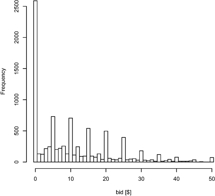
Figure A1. Histogram of the bids for the various products in the BDM task, using all the data.
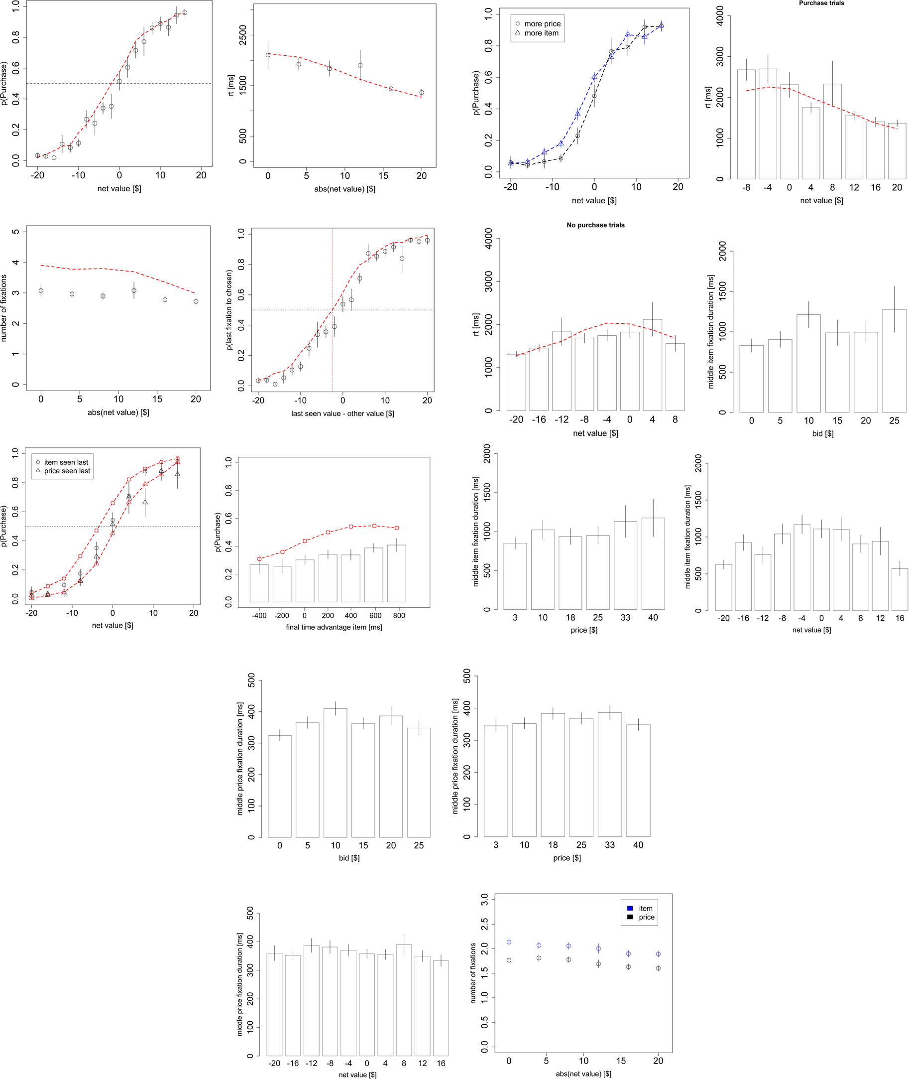
Figure A2. Replication of all the figures from the text but including the $0 products.
Figure A3. Replication of Figures 2A,B choice and reaction time curves but using all of the data, including the $0 bids and net values beyond +/−$20.
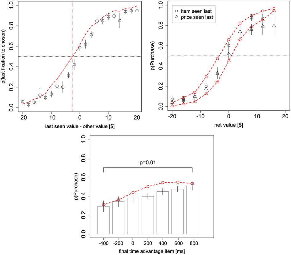
Figure A4. Replication of Figures 3A,B, and 4A but using both the even and odd-numbered trials.
Keywords: drift-diffusion, decision-making, neuroeonomics, decision neuroscience, eye-tracking, valuation, choice, purchasing
Citation: Krajbich I, Lu D, Camerer C and Rangel A (2012) The attentional drift-diffusion model extends to simple purchasing decisions. Front. Psychology 3:193. doi: 10.3389/fpsyg.2012.00193
Received: 15 February 2012; Accepted: 25 May 2012;
Published online: 13 June 2012.
Edited by:
Konstantinos Tsetsos, Oxford University, UKReviewed by:
Adele Diederich, Jacobs University Bremen, GermanyAndreas Glöckner, Max Planck Institute for Research on Collective Goods, Germany
Copyright: © 2012 Krajbich, Lu, Camerer and Rangel. This is an open-access article distributed under the terms of the Creative Commons Attribution Non Commercial License, which permits non-commercial use, distribution, and reproduction in other forums, provided the original authors and source are credited
*Correspondence: Antonio Rangel, Division of the Humanities and Social Sciences, California Institute of Technology, 1200 East California Boulevard, Pasadena, CA 91125, USA. e-mail: rangel@hss.caltech.edu